Bayes' Theorem: Updating Beliefs with Evidence

In 1763, Richard Price published a paper by his deceased friend Thomas Bayes. It contained a theorem that would take two centuries to appreciate.

Today, Bayes' theorem is everywhere. Spam filters. Medical diagnosis. Machine learning. Climate models. Legal reasoning. It's the mathematical rule for updating beliefs with evidence.

And it's surprisingly simple.

The Formula

Bayes' theorem:

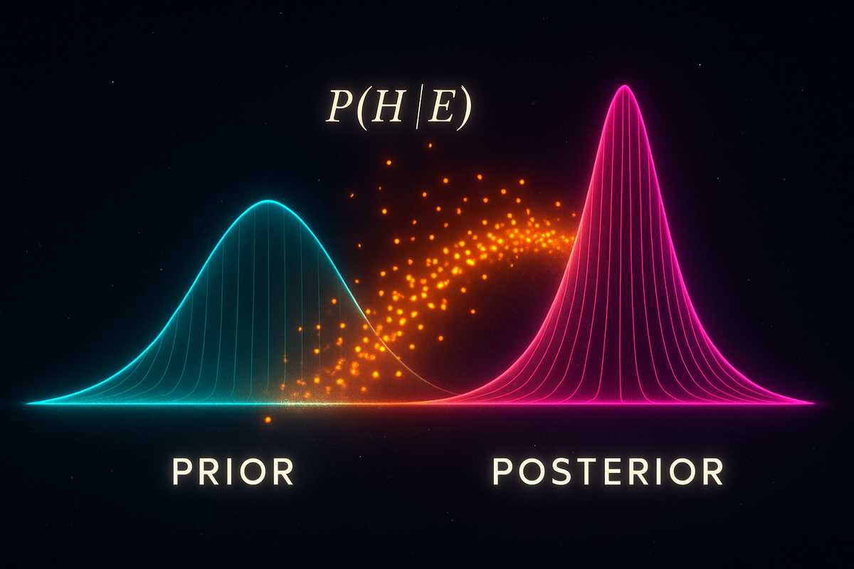
P(H | E) = P(E | H) × P(H) / P(E)

Where:

• H is a hypothesis
• E is evidence
• P(H) is the prior probability (what you believed before evidence)
• P(E | H) is the likelihood (how probable the evidence is if H is true)
• P(E) is the total probability of the evidence
• P(H | E) is the posterior probability (what you believe after evidence)

The theorem tells you how to update from prior to posterior when you observe evidence.

An Expanded Form

Often useful:

P(H | E) = P(E | H) × P(H) / [P(E | H) × P(H) + P(E | not H) × P(not H)]

The denominator expands P(E) using the law of total probability. This form makes all the pieces explicit.

The Intuition

Bayes' theorem is about reversing conditional probabilities.

We often know P(E | H)—how likely evidence is given a hypothesis. But we want P(H | E)—how likely the hypothesis is given the evidence.

Example: Medical testing.

We know: P(positive test | disease) = 0.99 (sensitivity) We want: P(disease | positive test)

These are very different! Bayes' theorem connects them.

Example: Crime investigation.

We know: P(DNA match | guilty) ≈ 1 We want: P(guilty | DNA match)

The theorem tells us the second depends critically on P(guilty) before the DNA evidence—the prior.

A Worked Example

A disease affects 1% of the population. A test has 90% sensitivity (true positive rate) and 90% specificity (true negative rate).

You test positive. What's the probability you have the disease?

Setting up:

• P(D) = 0.01 (prior: disease prevalence)
• P(not D) = 0.99
• P(+ | D) = 0.90 (sensitivity)
• P(+ | not D) = 0.10 (false positive rate = 1 - specificity)

Applying Bayes:

P(D | +) = P(+ | D) × P(D) / [P(+ | D) × P(D) + P(+ | not D) × P(not D)]

= (0.90 × 0.01) / (0.90 × 0.01 + 0.10 × 0.99)

= 0.009 / (0.009 + 0.099)

= 0.009 / 0.108

≈ 0.083 or 8.3%

A positive test only gives 8% probability of disease!

Why so low? Because the disease is rare. Most people testing positive don't have it—they're false positives from the large healthy population.

The Role of Priors

The prior P(H) is crucial. It's your belief before seeing evidence.

Same evidence, different priors:

If disease prevalence were 10% instead of 1%:

• P(D | +) jumps to about 50%

If prevalence were 50%:

• P(D | +) becomes about 90%

The rarer something is, the harder it is to confirm even with good tests.

Where do priors come from?

• Previous data (base rates in the population)
• Expert knowledge
• Other evidence
• Sometimes, reasonable assumptions when nothing else is available

Priors aren't arbitrary—they encode what you knew before this particular piece of evidence.

Sequential Updating

Evidence comes in sequence. Bayes' theorem handles this naturally.

Today's posterior becomes tomorrow's prior.

Example: Testing twice.

First positive test: P(D | +) = 0.083

If you test positive again:

• New prior: 0.083
• Same likelihood: P(+ | D) = 0.90, P(+ | not D) = 0.10

P(D | ++) = (0.90 × 0.083) / (0.90 × 0.083 + 0.10 × 0.917)

≈ 0.45

Two positive tests: about 45% probability.

Third positive test would push it higher. Each piece of evidence updates the probability.

Likelihood Ratios

A useful form:

Posterior odds = Likelihood ratio × Prior odds

Where:

• Odds = P(H) / P(not H)
• Likelihood ratio = P(E | H) / P(E | not H)

Example: The disease test.

Prior odds = 0.01 / 0.99 ≈ 0.0101 Likelihood ratio = 0.90 / 0.10 = 9

Posterior odds = 9 × 0.0101 ≈ 0.091 Posterior probability = 0.091 / 1.091 ≈ 0.083 ✓

This form shows: each piece of evidence multiplies your odds by the likelihood ratio. Strong evidence has high likelihood ratio; weak evidence has ratio near 1.

The Bayesian Worldview

Bayes' theorem is more than a formula. It's a philosophy of reasoning under uncertainty.

Beliefs as Probabilities:

Every proposition has a probability representing your degree of belief. Not whether it's true—you may not know that—but how confident you are.

Evidence Updates Beliefs:

When you observe something, you update beliefs using Bayes' theorem. Nothing is certain, but beliefs change rationally with evidence.

Priors Are Necessary:

You can't reason about evidence without prior beliefs. The theorem makes this explicit rather than hiding assumptions.

Coherence:

Bayesian reasoning is provably coherent—you can't be exploited by Dutch book bets if your beliefs follow Bayes' theorem.

Applications

Spam Filtering:

P(spam | words) is computed from P(words | spam), P(words | not spam), and prior spam rates. Naive Bayes classifiers use this directly.

Medical Diagnosis:

P(disease | symptoms) from P(symptoms | disease), disease prevalence, and symptom base rates. This is clinical reasoning formalized.

Machine Learning:

Bayesian neural networks maintain probability distributions over weights. Bayesian optimization chooses experiments efficiently. GPT-style models compute P(next word | previous words)—sequential Bayesian conditioning.

Legal Reasoning:

P(guilty | evidence) should be updated Bayesianly from P(evidence | guilty), priors based on base rates, and alternative explanations. Courts often get this wrong.

Science:

P(theory | data) is what scientists want. But experiments tell us P(data | theory). Bayes' theorem connects them. A theory that predicts surprising data (high likelihood ratio) gets strongly confirmed.

Common Errors

Ignoring Base Rates:

Focusing only on P(E | H) and ignoring P(H). This causes overconfidence in rare diagnoses.

Confusing P(H | E) with P(E | H):

The Prosecutor's Fallacy. P(evidence | innocent) isn't P(innocent | evidence).

Treating Priors as Bias:

Priors aren't illegitimate prejudice—they're required input. The question is whether they're reasonable.

Assuming 50-50 When Uncertain:

If you don't know, 50-50 isn't automatically right. A million hypotheses don't each get 50% probability.

Multiple Hypotheses

The full theorem handles any number of competing hypotheses:

P(Hᵢ | E) = P(E | Hᵢ) × P(Hᵢ) / Σⱼ P(E | Hⱼ) × P(Hⱼ)

Each hypothesis gets probability proportional to its prior times its likelihood.

Example: Three possible causes of a symptom.

• H₁: Common cold (prior 0.70, P(symptom | H₁) = 0.30)
• H₂: Flu (prior 0.25, P(symptom | H₂) = 0.60)
• H₃: Rare disease (prior 0.05, P(symptom | H₃) = 0.95)

P(E) = 0.30×0.70 + 0.60×0.25 + 0.95×0.05 = 0.21 + 0.15 + 0.0475 = 0.4075

P(H₁ | E) = 0.21 / 0.4075 ≈ 0.52 (cold most likely) P(H₂ | E) = 0.15 / 0.4075 ≈ 0.37 (flu possible) P(H₃ | E) = 0.0475 / 0.4075 ≈ 0.12 (rare disease unlikely despite high symptom probability)

The common cold wins despite lower symptom probability because it's much more common.

The Philosophical Stakes

Bayes' theorem answers a fundamental question: How should evidence change belief?

Before Bayes, there were intuitions about evidence being "strong" or "weak," but no calculus.

After Bayes, we have a formula. It tells us exactly how much a piece of evidence should shift probability, given what we knew before and what we learn.

This is one of humanity's greatest intellectual achievements: a mathematical solution to the problem of inductive reasoning.

The Pebble

Bayes' theorem is obvious once you see it:

P(A | B) = P(B | A) × P(A) / P(B)

It just rearranges P(A and B) = P(A | B) × P(B) = P(B | A) × P(A).

The profundity isn't in the mathematics. It's in the interpretation: prior belief + evidence = posterior belief.

The theorem doesn't tell you what to believe. It tells you how belief should update. If your beliefs don't update according to Bayes, they're inconsistent—and inconsistency leads to irrationality.

This simple formula is how to reason about uncertain things. Everything else is application.

This is Part 4 of the Probability series. Next: "Random Variables: Numbers from Chance."

Part 4 of the Probability series.

Previous: Conditional Probability: When Information Changes the Odds Next: Random Variables: Numbers That Depend on Chance