The Central Limit Theorem: Why the Bell Curve Rules
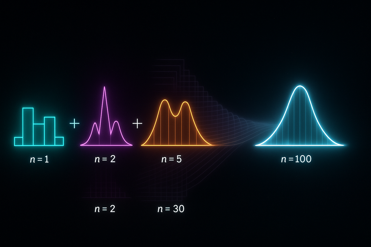
No matter what distribution your data come from, average enough independent samples and something remarkable happens: the averages form a bell curve. The Central Limit Theorem explains why normal distributions are everywhere.
The Central Limit Theorem (CLT) is arguably the most important theorem in statistics.
It says: the sum of many independent random variables is approximately normal—regardless of what distribution each variable has.
This explains why the bell curve appears everywhere. Any quantity that results from combining many small independent effects will be approximately normal.
The Statement
Let X₁, X₂, ..., Xₙ be independent random variables with the same distribution, mean μ, and finite variance σ².
Define the sample mean: X̄ₙ = (X₁ + ... + Xₙ) / n
Central Limit Theorem:
√n (X̄ₙ - μ) / σ → Normal(0, 1) as n → ∞
Equivalently: X̄ₙ is approximately Normal(μ, σ²/n) for large n.
The sample mean is approximately normal, centered at the true mean, with variance shrinking as 1/n.
What It Means
The original distribution doesn't matter. You could be summing Bernoulli trials, uniform random numbers, exponential waiting times—anything with finite variance. The sum becomes normal.
Approximation improves with n. The larger the sample, the better the normal approximation.
The normal has specific parameters. Mean = population mean. Variance = population variance / n.
Examples
Sum of Dice:
Roll a single die: discrete, uniform on {1, 2, 3, 4, 5, 6}. Not normal at all.
Roll two dice, sum them: peak at 7, roughly triangular. Still not normal.
Roll 10 dice, sum them: looks quite bell-shaped.
Roll 100 dice: almost perfectly normal.
The CLT in action.
Coin Flips:
Flip one coin: Bernoulli, 0 or 1. Not normal.
Flip 100 coins, count heads: approximately Normal(50, 25). You can use normal approximation for probabilities.
Sample Means:
Whatever your population distribution, sample means are approximately normal for large samples. This is why confidence intervals and hypothesis tests work.
Why It Works: Intuition
When you add random variables, you're convolving their distributions.
Convolution tends to "smooth out" distributions. Sharp edges get blurred. Bimodal peaks merge. The result becomes increasingly smooth and bell-shaped.
The normal distribution is the fixed point of convolution. It's the shape that adding produces, asymptotically.
Another view: adding random variables is like a random walk. Each step is independent. After many steps, the distribution of your position is determined by the geometry of random walks—which leads to the normal distribution.
The Role of Variance
Finite variance is required. If Var(X) = ∞, CLT fails.
The Cauchy distribution has infinite variance. Sum of Cauchy variables is still Cauchy, not normal. Fat tails don't smooth out.
This matters in finance. If returns have fat tails (infinite variance), normal-based models underestimate risk. The 2008 crisis involved such underestimation.
Speed of Convergence
How many samples for a good approximation?
It depends on the original distribution:
- Symmetric, low-kurtosis distributions: n = 20 often sufficient
- Skewed distributions: may need n = 50 or more
- Highly skewed or discrete: may need n = 100+
Berry-Esseen theorem: The error in the CLT approximation is O(1/√n). Converges, but slowly.
Rule of thumb: n ≥ 30 is often cited, but this is crude. Check skewness and kurtosis for better guidance.
Applications
Confidence Intervals:
The sample mean X̄ is approximately Normal(μ, σ²/n).
A 95% confidence interval for μ: X̄ ± 1.96 × (σ/√n)
This assumes the CLT approximation holds.
Hypothesis Testing:
Test whether a sample mean differs from a hypothesized value by computing a z-statistic:
z = (X̄ - μ₀) / (σ/√n)
Under the null hypothesis, z ≈ Normal(0, 1). Large |z| indicates deviation.
Quality Control:
Process means are monitored using control charts. The CLT justifies treating sample means as normal.
Polling:
A poll of n = 1000 voters estimates population proportion p.
Sample proportion p̂ is approximately Normal(p, p(1-p)/1000).
Margin of error ≈ 1.96 × √(p̂(1-p̂)/n) ≈ 3%.
Generalizations
Lindeberg-Lévy CLT: The basic version for i.i.d. samples.
Lindeberg-Feller CLT: For independent but not identically distributed variables, under conditions on variance.
Martingale CLT: For dependent sequences satisfying martingale conditions.
Multivariate CLT: For random vectors. The sum converges to multivariate normal.
Beyond Normal: When CLT Fails
Infinite variance: Fat-tailed distributions don't satisfy CLT. Sums follow stable distributions instead.
Strong dependence: If samples are highly correlated, CLT may not apply or may require modification.
Heavy tails: Power-law tails can lead to non-normal limits (stable distributions with infinite variance).
Example: Stock market returns have heavier tails than normal. The normal approximation works most of the time but fails for extreme events. This is why Value at Risk models sometimes fail catastrophically.
Relation to Law of Large Numbers
LLN: X̄ₙ → μ (convergence of location)
CLT: √n(X̄ₙ - μ) → Normal(0, σ²) (distribution of fluctuations)
LLN tells you where the sample mean goes. CLT tells you how it varies around that location.
LLN is about the point estimate. CLT is about uncertainty around the estimate.
Historical Development
De Moivre (1733): Showed binomial distribution approaches normal (a special case).
Laplace (1812): Extended to more general settings.
Lyapunov (1901): First rigorous general proof.
Lindeberg-Lévy (1920s): Modern statement and proof.
The CLT was understood empirically before it was proven. The bell curve kept appearing in astronomical observations, surveys, and experiments. The mathematics eventually caught up to explain why.
The Deep Insight
The CLT is a statement about universality.
Start with any distribution (finite variance). Add many copies. Get the normal distribution.
The normal isn't special because we chose it. It's special because it's the universal limit of addition. It's an attractor in the space of distributions.
This is why the bell curve appears in heights (sum of genetic effects), measurement errors (sum of noise sources), aggregate economic behavior (sum of individual decisions), and countless other contexts.
The normal distribution isn't assumed—it emerges.
This is Part 11 of the Probability series. Next: "Probability Synthesis: The Architecture of Uncertainty."
Part 11 of the Probability series.
Previous: The Law of Large Numbers: Why Averages Stabilize Next: Synthesis: Probability as the Logic of Uncertainty
Comments ()