Conditional Probability: When Information Changes the Odds

You're playing poker. Before you see your cards, the probability of having a flush is about 0.2%. Then you look: four hearts.

Now what's the probability of a flush?

Everything changed. Not the cards in the deck—your information about them. Conditional probability is the mathematics of this change.

What Conditional Probability Measures

The conditional probability of A given B, written P(A | B), is the probability of A happening when you know B has happened.

The formula:

P(A | B) = P(A and B) / P(B)

Read this as: of all the times B occurs, what fraction of those also have A?

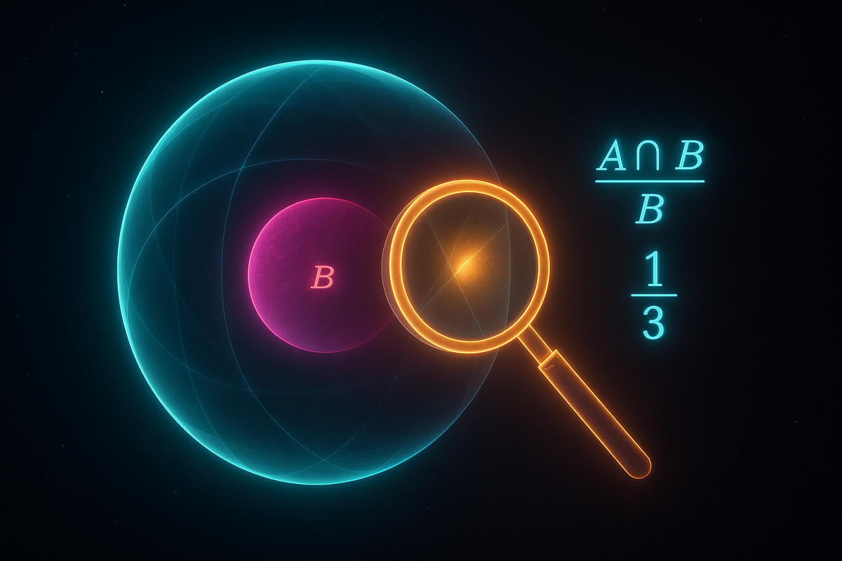
Visual intuition: Imagine the sample space as a rectangle. Event B is a region within it. Event A is another region. P(A | B) is the fraction of B that overlaps with A.

Once you know B happened, B becomes your new sample space. You're no longer in the full rectangle—you're in B. The conditional probability asks what fraction of B is also A.

The Definition in Action

Example 1: Cards

Draw one card from a standard deck. What's P(ace | face card)?

Face cards: J, Q, K of each suit. There are 12 face cards. Aces are not face cards.

P(ace | face card) = P(ace and face card) / P(face card) = 0 / (12/52) = 0

Knowing you have a face card eliminates any chance of an ace.

Example 2: Dice

Roll a fair die. What's P(6 | even)?

P(6 and even) = P(6) = 1/6 (6 is even) P(even) = 3/6 = 1/2

P(6 | even) = (1/6) / (1/2) = 1/3

Knowing the roll is even narrows possibilities to {2, 4, 6}. Among these, 6 is one of three.

Example 3: Families

A family has two children. You learn at least one is a boy. What's the probability both are boys?

Sample space: {BB, BG, GB, GG} "At least one boy": {BB, BG, GB} "Both boys": {BB}

P(both boys | at least one boy) = P(BB) / P(at least one boy) = (1/4) / (3/4) = 1/3

Wait—shouldn't it be 1/2? If one is a boy, isn't there a 50-50 chance the other is?

No. The information "at least one is a boy" doesn't specify which one. This matters.

If you instead learned "the older child is a boy," then: Given older is boy: {BB, BG} P(both boys | older is boy) = (1/4) / (1/2) = 1/2

How you get information changes the probability. This is the subtlety of conditioning.

The Chain Rule

From the definition, we can derive:

P(A and B) = P(A | B) × P(B)

This is the multiplication rule, restated. And it extends:

P(A and B and C) = P(A | B,C) × P(B | C) × P(C)

Any joint probability can be factored into a product of conditionals.

This is how language models work. They compute:

P(word₁, word₂, word₃, ...) = P(word₁) × P(word₂|word₁) × P(word₃|word₁,word₂) × ...

Each word's probability conditions on all previous words.

Independence Revisited

Two events are independent if:

P(A | B) = P(A)

Knowing B doesn't change A's probability. The information is irrelevant.

Equivalent formulations:

• P(A | B) = P(A)
• P(B | A) = P(B)
• P(A and B) = P(A) × P(B)

Example: Coin flips.

P(second flip heads | first flip heads) = P(second flip heads) = 1/2

The first flip doesn't affect the second. Independent.

Example: Drawing cards without replacement.

P(second ace | first ace) = 3/51 ≠ P(second ace) = 4/52

Dependent. First draw affects what's available.

The Prosecutor's Fallacy

Conditional probability has a dangerous trap.

P(A | B) is NOT the same as P(B | A).

Example: A crime scene has DNA matching 1 in a million people. The defendant's DNA matches.

P(match | innocent) = 1/1,000,000

But the prosecutor argues: "There's only a one-in-a-million chance of innocence!"

This confuses P(match | innocent) with P(innocent | match).

If there are 10 million potential suspects, about 10 would match by chance. The defendant is one of perhaps 10 people with matching DNA. P(innocent | match) could be as high as 9/10.

The fallacy: assuming P(A|B) = P(B|A). They're often very different.

The Base Rate Problem

A disease affects 1 in 10,000 people. A test is 99% accurate (99% true positive rate, 99% true negative rate).

You test positive. What's the probability you have the disease?

Most people guess around 99%. The real answer: about 1%.

Let's work it out with 1 million people:

• 100 have the disease (1 in 10,000)
• 99 of those test positive (99% true positive)
• 999,900 don't have it
• 9,999 of those test positive (1% false positive)

Total positives: 99 + 9,999 = 10,098 True positives: 99 P(disease | positive) = 99 / 10,098 ≈ 1%

The base rate (1 in 10,000) dominates. Even accurate tests produce mostly false positives when the condition is rare.

This is the base rate fallacy. Ignoring prior probability leads to wildly wrong conclusions.

The Reverend's Theorem

How do you compute P(B | A) when you know P(A | B)?

Enter Bayes' theorem:

P(B | A) = P(A | B) × P(B) / P(A)

This reverses the conditioning. We'll cover it fully in the next article, but here's the essence:

P(cause | effect) = P(effect | cause) × P(cause) / P(effect)

We observe effects and want to infer causes. Bayes' theorem is the tool.

Conditional Probability in Practice

Medical Diagnosis:

P(disease | symptoms) = P(symptoms | disease) × P(disease) / P(symptoms)

Symptoms are observed. We want to know diseases. Medicine constantly inverts conditional probabilities.

Spam Filters:

P(spam | contains "Nigerian prince") is what we want. We know P(contains "Nigerian prince" | spam). Bayes' theorem converts one to the other.

Machine Learning:

Classification is computing P(class | features). We train on examples that tell us P(features | class). Bayes' theorem connects them.

Evidence and Belief:

P(hypothesis | evidence) is what we want. P(evidence | hypothesis) is what experiments tell us. Bayes' theorem is how evidence updates belief.

The Geometry of Conditioning

Here's a visual way to think about conditional probability:

Imagine the sample space as a circle with area 1. Events are regions within it. P(A) is A's area.

When you condition on B, you're zooming in on B. B becomes your new universe. Areas rescale so B has area 1.

P(A | B) is A's area after zooming into B.

This explains why P(A | B) = P(A and B) / P(B). You're measuring the intersection, but normalizing by B's area (since B is now the whole space).

Conditional Independence

Events A and B can be dependent in general but independent given C.

Example: Two witnesses testify. Their testimonies seem correlated—both agree on what happened.

In general, P(witness 2 agrees | witness 1 agrees) > P(witness 2 agrees).

But given the truth of what happened: P(witness 2 agrees | witness 1 agrees and truth) = P(witness 2 agrees | truth)

Conditioned on the actual event, their agreements are independent—they're each responding to reality, not to each other.

Formally: A and B are conditionally independent given C if: P(A and B | C) = P(A | C) × P(B | C)

Conditional independence is central to probabilistic graphical models in machine learning.

Traps and Clarifications

Trap 1: P(A | B) doesn't mean B causes A. It means knowing B changes our assessment of A's likelihood.

Trap 2: P(A | B) ≠ P(B | A) in general. The reversal requires Bayes' theorem.

Trap 3: Conditioning isn't intervention. P(lung cancer | yellow teeth) is high, but brushing your teeth doesn't prevent lung cancer. Smoking causes both.

Trap 4: "Given" has precise meaning. P(heads | coin is fair) = 0.5 treats coin fairness as known. P(heads | I believe coin is fair) might be different—your belief could be wrong.

The Core Insight

Conditional probability is about restricting your universe.

When you learn B happened, you're no longer asking about all possibilities—you're asking about possibilities consistent with B.

This restriction is not just a mathematical formality. It's how updating works. Every time you learn something, you condition. Every observation narrows the possibilities.

Probability before evidence. Probability after evidence. The mathematics of moving between them is conditional probability and its culmination: Bayes' theorem.

This is Part 3 of the Probability series. Next: "Bayes' Theorem: The Mathematics of Belief."

Part 3 of the Probability series.

Previous: Basic Probability Rules: And Or and Not Next: Bayes' Theorem: Updating Beliefs with Evidence