Definite Integrals: Computing Exact Areas

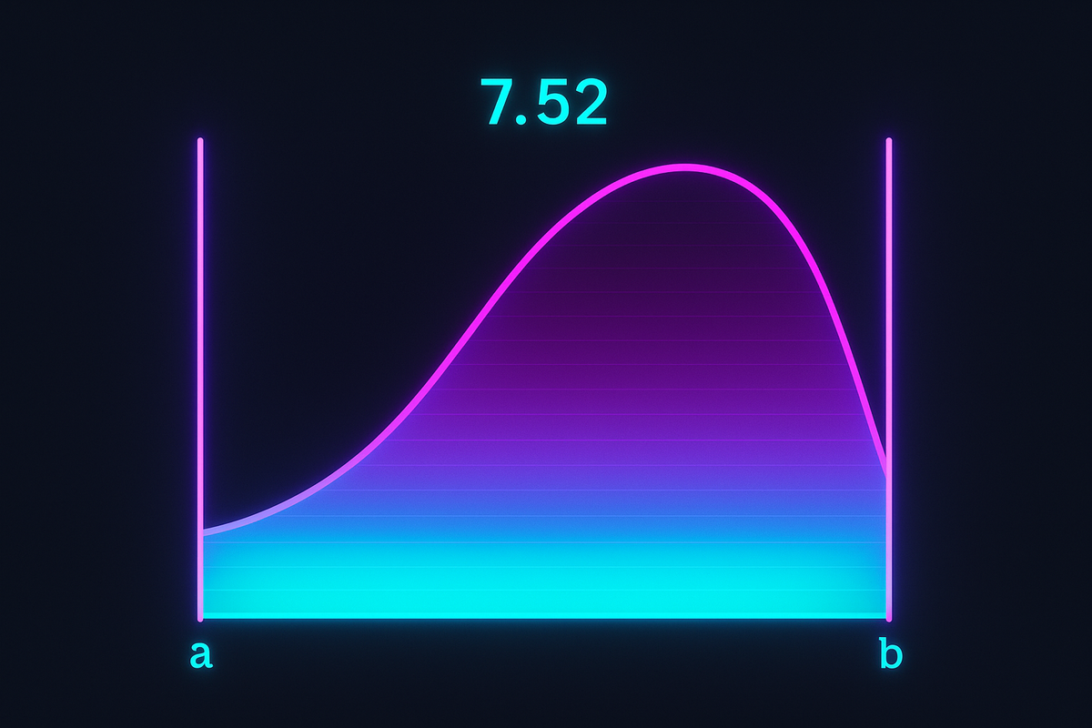
A definite integral gives you a number, not a function.

Where indefinite integrals answer "what function has this derivative?", definite integrals answer "what is the total accumulation between these bounds?"

The result is specific, concrete, computable. Not F(x) + C. Just a number.

The Definition

The definite integral from a to b is:

∫ₐᵇ f(x) dx

Two interpretations, both valid:

1. Area: The signed area between f(x), the x-axis, and the vertical lines x = a and x = b.
2. Accumulation: The total accumulation of f(x) over the interval [a, b].

The Fundamental Theorem connects this to antiderivatives:

∫ₐᵇ f(x) dx = F(b) - F(a)

where F'(x) = f(x).

Signed Area

The integral counts area with sign.

• Area above the x-axis contributes positive.
• Area below the x-axis contributes negative.

This is crucial. If you integrate sin(x) from 0 to 2π, you get zero — not because there's no area, but because the positive and negative regions cancel.

∫₀^(2π) sin(x) dx = [-cos(x)]₀^(2π) = (-cos(2π)) - (-cos(0)) = -1 - (-1) = 0

If you want total area regardless of sign, integrate |f(x)| instead:

∫₀^(2π) |sin(x)| dx = 4

Computing Definite Integrals

Step 1: Find an antiderivative F(x) of f(x).

Step 2: Evaluate at bounds: F(b) - F(a).

Step 3: The constant C cancels, so ignore it.

Example: ∫₁³ (2x + 1) dx

Antiderivative: F(x) = x² + x

Evaluate: F(3) - F(1) = (9 + 3) - (1 + 1) = 12 - 2 = 10.

That's the area under y = 2x + 1 from x = 1 to x = 3.

Properties of Definite Integrals

Linearity: ∫ₐᵇ [f(x) + g(x)] dx = ∫ₐᵇ f(x) dx + ∫ₐᵇ g(x) dx ∫ₐᵇ k·f(x) dx = k · ∫ₐᵇ f(x) dx

Additivity over intervals: ∫ₐᵇ f(x) dx + ∫ᵦᶜ f(x) dx = ∫ₐᶜ f(x) dx

Integrate in pieces, add results. This is how you handle functions that change behavior.

Reversing limits: ∫ₐᵇ f(x) dx = -∫ᵦᵃ f(x) dx

Swapping a and b negates the integral. Area traversed "backward" is negative.

Zero-width integral: ∫ₐᵃ f(x) dx = 0

No interval, no area.

Geometric Examples

Triangle: f(x) = x from 0 to 2.

∫₀² x dx = [x²/2]₀² = 4/2 - 0 = 2

Check: Triangle with base 2, height 2 has area ½ · 2 · 2 = 2. ✓

Rectangle: f(x) = 3 from 1 to 5.

∫₁⁵ 3 dx = [3x]₁⁵ = 15 - 3 = 12

Check: Rectangle with width 4, height 3 has area 4 · 3 = 12. ✓

Parabola: f(x) = x² from 0 to 1.

∫₀¹ x² dx = [x³/3]₀¹ = 1/3 - 0 = 1/3

No simple geometric check, but calculus handles it effortlessly.

Average Value

The average value of f(x) on [a, b] is:

f_avg = (1/(b-a)) · ∫ₐᵇ f(x) dx

This is the height of a rectangle with the same area as the region under f.

Example: Average value of x² on [0, 3].

∫₀³ x² dx = [x³/3]₀³ = 9

f_avg = (1/3) · 9 = 3

On [0, 3], the average value of x² is 3.

When Antiderivatives Are Hard

Not every definite integral requires finding F(x) explicitly.

Numerical methods: Simpson's rule, trapezoidal rule, and computer algorithms can approximate ∫ₐᵇ f(x) dx to any desired precision.

Symmetry: If f is odd and the interval is symmetric about 0, the integral is 0.

∫₋₂² x³ dx = 0 (x³ is odd)

Comparison: If you can bound f(x), you can bound its integral.

If 0 ≤ f(x) ≤ g(x) on [a, b], then: 0 ≤ ∫ₐᵇ f(x) dx ≤ ∫ₐᵇ g(x) dx

The Mean Value Theorem for Integrals

If f is continuous on [a, b], there exists some c in (a, b) such that:

f(c) = (1/(b-a)) · ∫ₐᵇ f(x) dx

The function achieves its average value somewhere in the interval.

Geometrically: there's a horizontal line at height f(c) such that the rectangle it forms has the same area as the region under the curve.

Definite Integrals as Functions of Bounds

Define:

A(x) = ∫ₐˣ f(t) dt

This is a function of x — the accumulated area from a to x.

By the Fundamental Theorem (Part 1):

A'(x) = f(x)

The rate at which area accumulates equals the function value.

This perspective is key for variable limits and differential equations.

Substitution with Definite Integrals

When you substitute u = g(x), the bounds change too.

∫ₐᵇ f(g(x)) · g'(x) dx = ∫_{g(a)}^{g(b)} f(u) du

Example: ∫₀¹ 2x · e^(x²) dx

Let u = x². Then du = 2x dx. When x = 0: u = 0. When x = 1: u = 1.

∫₀¹ 2x · e^(x²) dx = ∫₀¹ eᵘ du = [eᵘ]₀¹ = e - 1

The bounds transform with the substitution. You never go back to x.

Common Pitfalls

Forgetting sign: ∫₋₁¹ x³ dx = 0, not some positive value.

Odd functions integrate to zero over symmetric intervals.

Ignoring where f is negative: ∫₀^(2π) sin(x) dx = 0, but total area is 4.

For total unsigned area, integrate |f(x)|.

Substitution bounds: After substitution, use new bounds. Don't substitute u back to x and then use old bounds.

Physical Applications

Distance from velocity: If v(t) is velocity, then ∫ₜ₁^(t₂) v(t) dt is displacement from t₁ to t₂.

Work from force: If F(x) is force as a function of position, then ∫ₐᵇ F(x) dx is work done.

Total charge from current: If I(t) is current, then ∫₀ᵀ I(t) dt is total charge transferred.

The integral of a rate equals the total change. This is the physical meaning of the Fundamental Theorem.

Further Reading

• Thomas, G. & Finney, R. Calculus and Analytic Geometry. Excellent worked examples.
• Apostol, T. Calculus, Vol. 1. Rigorous treatment.
• MIT OpenCourseWare 18.01 — Free calculus lectures with problems.

This is Part 4 of the Integrals series. Next: "U-Substitution" — the most common integration technique.

Part 4 of the Calculus Integrals series.

Previous: Indefinite Integrals: Finding Antiderivatives Next: U-Substitution: The Chain Rule in Reverse