Differential Equations: When Derivatives and Functions Mix

A differential equation is an equation where the unknown is a function, and the equation involves that function's derivatives.

Instead of solving for x, you solve for y(x) — an entire function, not just a number.

This is where calculus becomes physics, biology, economics, and engineering. Differential equations model change. And everything changes.

What Is a Differential Equation?

An ordinary differential equation (ODE) is an equation involving a function and its derivatives.

Examples:

dy/dx = 2x — the derivative of y equals 2x. dy/dx = y — the derivative equals the function itself. d²y/dx² + y = 0 — involves the second derivative. dy/dx = y(1 - y) — the logistic equation.

The goal: find all functions y(x) that satisfy the equation.

Why They Matter

Derivatives describe rates of change. Differential equations describe how rates relate to quantities.

• Newton's second law: F = ma means m(d²x/dt²) = F(x,t). This is a differential equation for position.
• Radioactive decay: The decay rate is proportional to the amount present. dN/dt = -λN.
• Population growth: Growth rate depends on population size. dP/dt = rP(1 - P/K).
• Compound interest (continuous): dA/dt = rA.

Any time a rate depends on the current state, you have a differential equation.

The Simplest Case: dy/dx = f(x)

When the equation is dy/dx = f(x), just integrate:

y = ∫ f(x) dx + C

The solution is any antiderivative of f.

Example: dy/dx = 3x². Then y = x³ + C.

This is why integration is "solving the simplest differential equation."

Exponential Growth: dy/dx = ky

The equation dy/dx = ky says: the rate of change is proportional to the current value.

What function has a derivative proportional to itself?

The exponential: y = Ce^(kx).

Check: dy/dx = Cke^(kx) = k · Ce^(kx) = ky ✓

Every function satisfying dy/dx = ky is an exponential.

When k > 0: exponential growth. When k < 0: exponential decay.

This is why exponentials appear everywhere — population, radioactivity, interest, epidemics.

Separation of Variables

For equations of the form dy/dx = f(x)g(y), separate variables:

dy/g(y) = f(x) dx

Then integrate both sides.

Example: dy/dx = xy

Separate: dy/y = x dx

Integrate: ln|y| = x²/2 + C

Solve for y: y = Ae^(x²/2), where A = ±e^C.

Example: dy/dx = y²

Separate: dy/y² = dx

Integrate: -1/y = x + C

Solve: y = -1/(x + C)

Initial Value Problems

A differential equation typically has infinitely many solutions (the constant C can be anything).

An initial condition specifies the function's value at one point: y(x₀) = y₀.

This determines C, giving a unique solution.

Example: dy/dx = 2y, y(0) = 5.

General solution: y = Ce^(2x).

Apply initial condition: y(0) = Ce⁰ = C = 5.

Particular solution: y = 5e^(2x).

First-Order Linear Equations

The general first-order linear ODE:

dy/dx + P(x)y = Q(x)

This can always be solved using an integrating factor.

Multiply by μ(x) = e^(∫P(x)dx):

d/dx[μy] = μQ

Then integrate: μy = ∫ μQ dx.

Example: dy/dx + 2y = e^(-x).

P(x) = 2, so μ = e^(2x).

Multiply: e^(2x) dy/dx + 2e^(2x) y = e^x

This is d/dx[e^(2x) y] = e^x.

Integrate: e^(2x) y = e^x + C.

Solve: y = e^(-x) + Ce^(-2x).

Second-Order Equations: A Preview

The equation d²y/dx² + y = 0 (simple harmonic motion) involves the second derivative.

Solutions are y = A cos(x) + B sin(x).

Two constants appear because it's second-order — you need two initial conditions (position and velocity) to pin down the solution.

This describes springs, pendulums, circuits, and anything that oscillates.

The full treatment requires more machinery (characteristic equations, Wronskians), covered in a dedicated differential equations course.

Existence and Uniqueness

Does every differential equation have a solution? Is it unique?

Existence: Under mild conditions (f continuous), solutions exist locally.

Uniqueness: If additionally ∂f/∂y exists and is continuous, then for any initial condition, there's exactly one solution.

Some equations violate these conditions:

dy/dx = √y, y(0) = 0 has infinitely many solutions (y = 0 and y = (x/2)² for x ≥ 0 both work).

But for most "nice" equations, existence and uniqueness hold.

Numerical Solutions

Many differential equations can't be solved analytically.

Euler's method: Approximate by stepping along the tangent line.

Start at (x₀, y₀). At each step: y_{n+1} = y_n + f(x_n, y_n) · Δx x_{n+1} = x_n + Δx

This traces out an approximate solution curve.

More sophisticated methods (Runge-Kutta) give better accuracy.

Computer simulations of weather, economics, and physics all rely on numerical ODE solvers.

The Logistic Equation

dP/dt = rP(1 - P/K)

This models population with carrying capacity K.

• Small P: approximately dP/dt = rP (exponential growth)
• P near K: growth slows
• P = K: dP/dt = 0 (equilibrium)

Solution: P(t) = K / (1 + Ae^(-rt)), a sigmoid curve.

This appears in ecology, epidemiology (SIR model), and technology adoption.

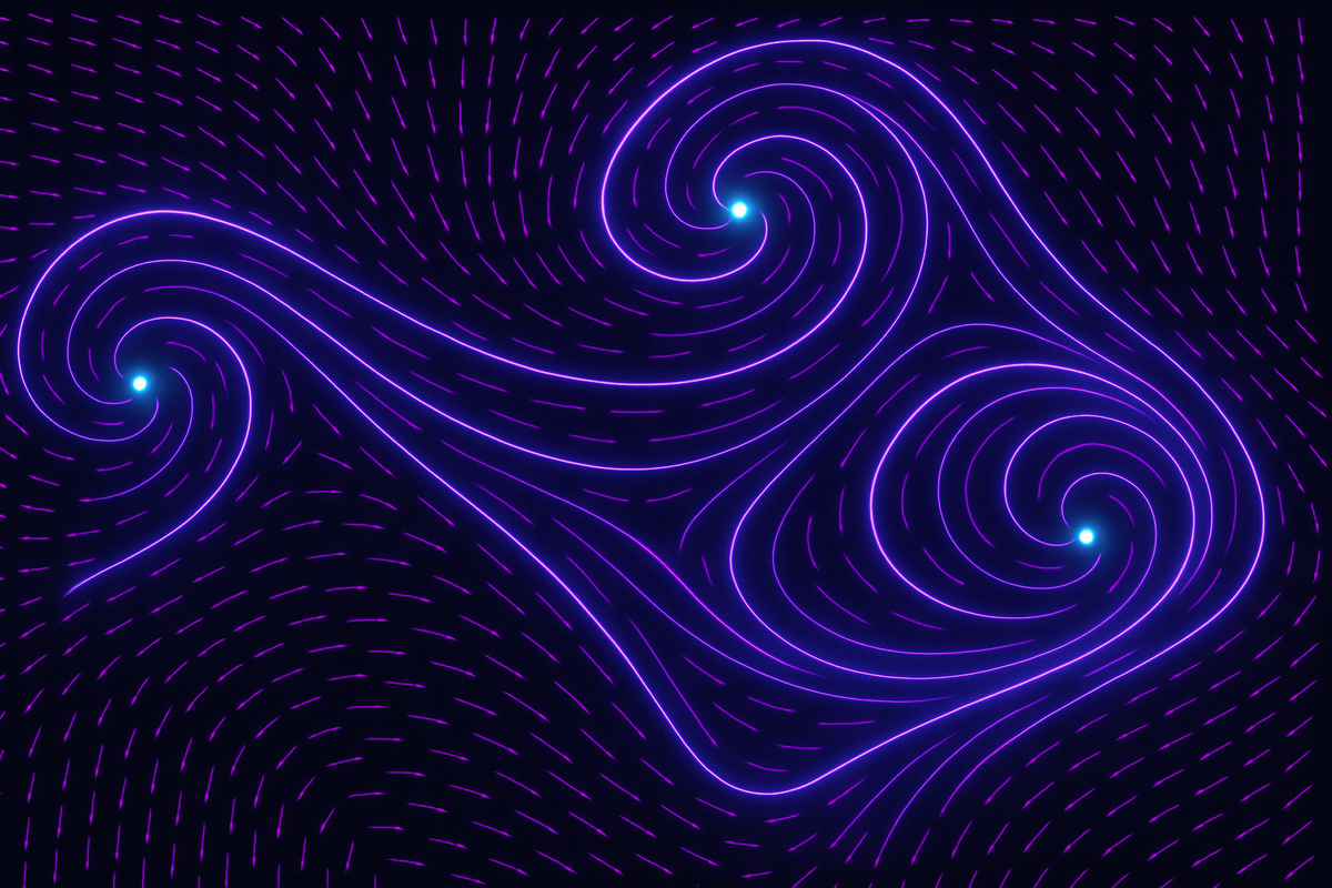
Direction Fields

Even without solving, you can visualize an ODE.

A direction field plots a small line segment at each point (x, y) with slope f(x, y).

Solution curves are tangent to these segments everywhere.

Sketching direction fields reveals qualitative behavior: equilibria, stability, trajectories.

This is the geometric heart of differential equations.

The Big Picture

Differential equations are how mathematics describes dynamical systems — anything that evolves according to rules.

Integration is the simplest case: find y from dy/dx.

Separation of variables, integrating factors, and other techniques extend this to more complex relationships.

When exact solutions fail, numerical methods and qualitative analysis take over.

Every physics equation, every biological model, every economic simulation runs on differential equations. This is where pure mathematics meets the real world.

Further Reading

• Boyce & DiPrima. Elementary Differential Equations. The standard text.
• Strogatz, S. Nonlinear Dynamics and Chaos. Qualitative and geometric approach.
• MIT OCW 18.03 — Full differential equations course free online.

This is Part 9 of the Integrals series. Next: "Synthesis: The Language of Totals" — what integration really means.

Part 9 of the Calculus Integrals series.

Previous: Applications of Integration: Volume Area and Arc Length Next: Synthesis: The Integral as the Language of Totals