Synthesis: Differential Equations as the Grammar of Physics
Almost every fundamental law in physics is a differential equation in disguise. Mastering that grammar means reading the deep structure of how systems evolve — from pendulums to quantum fields.
Differential equations describe change. Everything we've covered—from first-order separation to Laplace transforms—is a toolkit for translating dynamic reality into mathematical form and extracting predictions.
Let's synthesize. How does it all connect? Why does it matter? What's the deeper structure?
The Central Pattern: Local Rules → Global Behavior
Every differential equation embodies the same pattern:
Specify local dynamics (how things change instant to instant) → Derive global trajectories (how things evolve over time).
You don't need to know the full solution in advance. You just need to know the rules governing change. The trajectory emerges from iterating those rules.
This is profound. You can describe complex phenomena without explicit formulas—just local relationships.
Newton didn't need to know the trajectory of a falling apple. He just needed F = ma and F = -mg. The parabola emerges.
Maxwell didn't need to know what electromagnetic waves "are." He just needed relationships between electric and magnetic fields. Light emerges as a wave solution.
Schrödinger didn't need to visualize electron orbitals. He just needed the relationship between energy and wavefunction. Atomic structure emerges.
Differential equations are generative. They produce complexity from simplicity.
The Hierarchy of Difficulty
Not all differential equations are created equal. There's a natural hierarchy:
Level 1: First-Order Linear
dy/dx + P(x)y = Q(x)
Method: Integrating factor.
Complexity: Low. Systematic, always solvable.
Examples: Exponential growth/decay, Newton's cooling, RC circuits.
Level 2: First-Order Separable/Bernoulli
dy/dx = g(x)h(y) or dy/dx + P(x)y = Q(x)y^n
Method: Separation of variables, substitution.
Complexity: Medium. Solvable if integrals are computable.
Examples: Logistic growth, mixing problems, population with harvesting.
Level 3: Second-Order Linear Constant Coefficient
ay'' + by' + cy = f(x)
Method: Characteristic equation, undetermined coefficients, variation of parameters.
Complexity: Medium-high. Homogeneous part systematic, particular solution requires technique matching.
Examples: Harmonic oscillator, damped vibration, RLC circuits.
Level 4: Systems of Linear ODEs
dX/dt = AX
Method: Eigenvalue decomposition, matrix exponential.
Complexity: High. Requires linear algebra, eigenvalue computation.
Examples: Coupled oscillators, predator-prey (linearized), multi-component mixing.
Level 5: Nonlinear ODEs and Systems
dy/dx = f(x, y) where f is nonlinear, or nonlinear systems
Method: Linearization near equilibria, phase plane analysis, numerics.
Complexity: Very high. Analytical solutions rare; chaos possible.
Examples: Pendulum (exact), Lorenz system, Van der Pol oscillator, nonlinear population models.
Level 6: Partial Differential Equations
∂u/∂t = f(u, ∂u/∂x, ∂²u/∂x², ...)
Method: Separation of variables, Fourier/Laplace transforms, numerical PDE solvers.
Complexity: Extreme. Higher-dimensional, boundary conditions critical, computationally intensive.
Examples: Heat equation, wave equation, Navier-Stokes, Schrödinger equation.
Mastery path: Start at Level 1, build up. Each level requires the previous as foundation.
The Toolkit: When to Use What
| Equation Type | Method | Key Idea |
|---|---|---|
| First-order separable | Separation of variables | Factor into g(x)h(y), integrate separately |
| First-order linear | Integrating factor | Multiply by μ(x) to make left side a derivative |
| Bernoulli | Substitution v = y^(1-n) | Transform to linear |
| Second-order homogeneous | Characteristic equation | Try e^(rx), solve polynomial |
| Second-order nonhomogeneous | Undetermined coefficients / Variation of parameters | Find y_c + y_p |
| Systems (linear) | Eigenvalues | Diagonalize, solve decoupled |
| Nonlinear | Linearization + numerics | Jacobian near equilibria, RK4 for trajectories |
| Any ODE (numeric) | Euler / RK4 | Step through slope field |
| Linear with complex forcing | Laplace transform | Convert to algebra, transform back |
Strategy: Identify equation type → select method → apply technique.
The Deep Structures
Beneath the variety of methods, certain structures recur:
Superposition (Linearity)
For linear equations, solutions add:
If y₁ and y₂ solve the homogeneous equation, so does C₁y₁ + C₂y₂.
This is why linear equations are tractable. The solution space is a vector space.
Nonlinear equations don't have this. Solutions don't add. You can't build general solutions from particular ones.
Exponentials as Eigenfunctions
Why do exponentials appear everywhere?
Because differentiation is a linear operator, and exponentials are its eigenfunctions:
d/dx[e^(rx)] = re^(rx)
Differentiating multiplies by r. This is eigenvalue behavior: L[φ] = λφ.
For linear constant-coefficient ODEs, eigenfunctions are exponentials (or exponentials times trig, which are also exponentials in complex form).
This is why the characteristic equation works. It finds eigenvalues of the differential operator.
Stability from Eigenvalues
For systems dX/dt = AX, stability is determined by eigenvalues of A:
- All Re(λ) < 0: stable (decay to equilibrium)
- Any Re(λ) > 0: unstable (divergence)
- Re(λ) = 0: marginal (oscillation, no decay)
Eigenvalues encode asymptotic behavior. The system is a vector field, eigenvalues describe flow.
Conservation and Invariants
Some systems conserve quantities.
Energy conservation: Hamiltonian systems conserve H(x, y).
Mass conservation: Chemical systems conserve total concentration.
Probability conservation: Quantum mechanics conserves ∫|ψ|² dx = 1.
Conserved quantities constrain dynamics. They're first integrals—functions constant along trajectories.
Finding conserved quantities can simplify or completely solve systems.
Real-World Applications Recap
Differential equations aren't abstract. They're the language of:
Physics
- Mechanics: F = ma →
m(d²x/dt²) = F - Electromagnetism: Maxwell's equations (PDEs)
- Thermodynamics: Heat equation, diffusion
- Quantum mechanics: Schrödinger equation
- Relativity: Geodesic equations, Einstein field equations
Every physical law is a differential equation or system thereof.
Biology
- Population dynamics: Logistic equation, predator-prey
- Epidemic spread: SIR models
- Neural firing: Hodgkin-Huxley equations
- Biochemical reactions: Michaelis-Menten kinetics
- Pattern formation: Reaction-diffusion (Turing patterns)
Living systems are dynamic. Differential equations model growth, interaction, adaptation.
Engineering
- Control systems: Transfer functions, feedback loops
- Circuits: RLC equations, Kirchhoff's laws
- Structural mechanics: Vibration, resonance
- Fluid dynamics: Navier-Stokes equations
- Signal processing: Filtering, convolution
Engineering is applied differential equations. Design requires predicting dynamic behavior.
Economics and Social Science
- Growth models: Solow model (capital accumulation)
- Market dynamics: Supply-demand equilibrium
- Diffusion of innovations: Bass model
- Opinion dynamics: Voter models
Even social systems exhibit dynamics describable by differential equations (with caveats about stochasticity and human agency).
The Limits of Differential Equations
Differential equations are powerful but not omnipotent.
When They Fail
Stochasticity: Differential equations are deterministic. Real systems have noise. Solution: Stochastic differential equations (SDEs) add random terms.
Discrete events: Differential equations assume continuity. Some systems have jumps (e.g., population of integer organisms). Solution: Difference equations, discrete-time models.
Discontinuities: Some forcing functions are wildly discontinuous. Solution: Distributions (delta functions), weak solutions.
Chaos: Some systems are unpredictable despite being deterministic. Tiny initial condition errors blow up exponentially. Solution: Statistical description, ensemble methods.
Complexity: Some systems (e.g., full brain, climate) are too complex for analytical solutions. Solution: Numerical simulation, data-driven modeling, reduced-order models.
The Computational Turn
Most real-world differential equations can't be solved analytically. Numerical methods dominate:
- Simulation: Integrate ODEs/PDEs numerically (RK4, finite elements, spectral methods)
- Parameter estimation: Fit models to data
- Uncertainty quantification: Propagate input uncertainty through simulations
- Machine learning: Neural networks approximate solutions (PINNs—physics-informed neural networks)
The 21st century approach: combine mathematical structure (differential equations) with computational power.
The Philosophical Core
Why do differential equations work so well?
Because the universe is local and causal.
Physical laws relate nearby states and times. What happens at (x, t) depends on what's happening infinitesimally close to (x, t).
Derivatives capture this locality. df/dx is the limit as Δx → 0. It's the instantaneous, the local, the causal.
Differential equations say: "The future is determined by the present and the local rules of change."
This is why they're universal. Locality + causality → differential structure.
What You've Learned
You now have:
- Conceptual foundation: What differential equations are, why they matter, how they model reality.
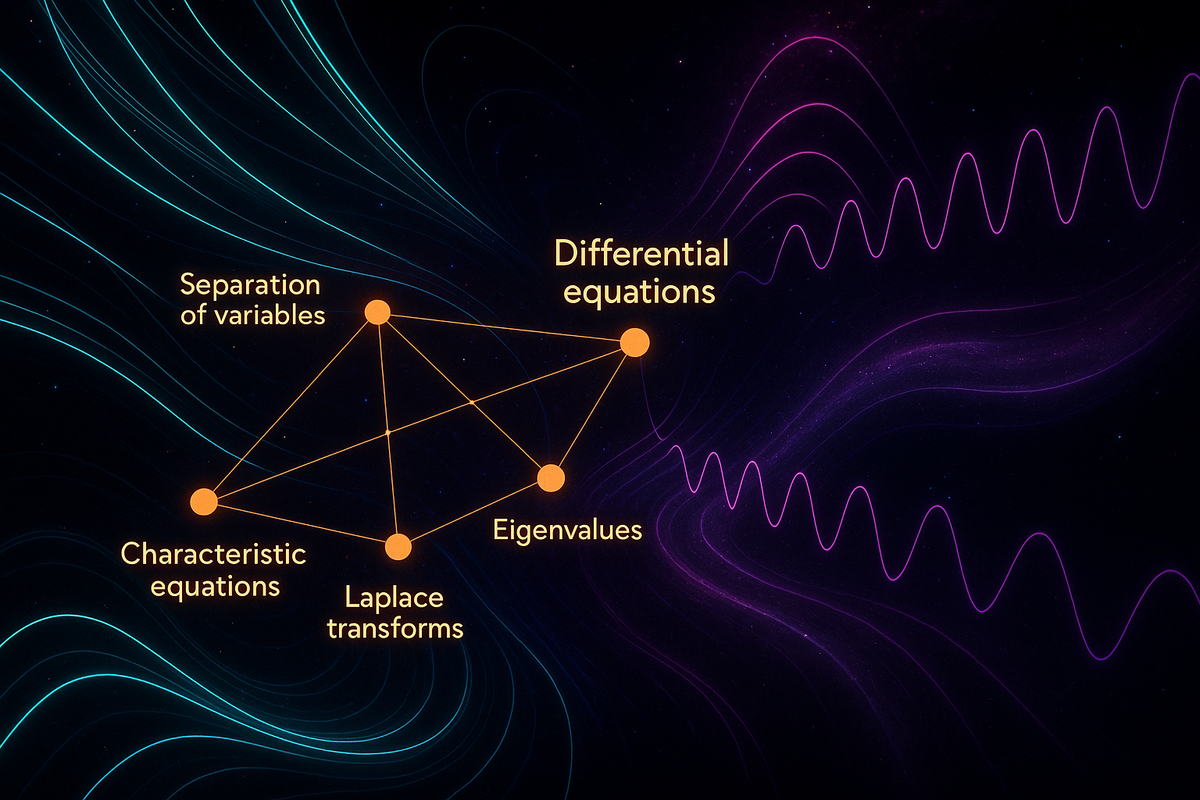
- Technical methods: Separation, integrating factor, characteristic equation, eigenvalues, Laplace transforms, numerics.
- Structural insight: Linearity, stability, eigenvalues, conservation laws, phase space.
- Applications: Physics, biology, engineering, real systems modeled by ODEs.
You can recognize equation types and select appropriate methods. You can interpret solutions physically. You can analyze stability and long-term behavior.
Most importantly: you understand that differential equations are the mathematics of change.
Where to Go Next
This series covered ODEs—ordinary differential equations. The natural extensions:
Partial Differential Equations (PDEs): Heat, wave, Laplace, Schrödinger equations. Essential for fields, continua, spatial dynamics.
Stochastic Differential Equations (SDEs): Add randomness. Critical for finance, molecular dynamics, noisy systems.
Dynamical Systems Theory: Qualitative analysis, bifurcations, chaos, attractors. Understand behavior without solving.
Numerical Methods: Finite differences, finite elements, spectral methods. Computational differential equations.
Functional Analysis: Infinite-dimensional spaces, operator theory. Rigorous foundation for PDEs and quantum mechanics.
Control Theory: Designing systems with desired dynamic behavior. Feedback, stability, optimal control.
Each is a deep field. Differential equations are the gateway.
The Unifying Vision
Across all the techniques—separation, integrating factors, eigenvalues, Laplace—the core remains:
Differential equations encode how things change. Solutions describe how things evolve.
From the decay of radioactive atoms to the orbit of planets to the spread of ideas, the mathematics is the same: relate the rate of change to the current state, then solve for the trajectory.
It's the mathematics of time, motion, and transformation. Of becoming rather than being.
Master differential equations, and you master the language of dynamics.
And dynamics is the heart of reality.
Part 12 of the Differential Equations series.
Previous: The Laplace Transform: Turning Calculus into Algebra
Comments ()