Directional Derivatives: Rates of Change in Any Direction

Partial derivatives tell you how a function changes along coordinate axes. The gradient tells you the direction of steepest ascent. But what if you want to know the rate of change in some other direction—diagonally, along a curve, at an arbitrary angle?

That's what directional derivatives capture: the rate of change of a function in any direction you specify.

This completes the picture of multivariable differentiation. Partial derivatives are directional derivatives in special directions (along axes). The gradient is the directional derivative of maximum magnitude (steepest slope). Once you understand directional derivatives, you have the full toolkit for analyzing how functions vary in multidimensional space.

The Setup: Specifying a Direction

In single-variable calculus, there's only one direction to move: forward (increasing x) or backward (decreasing x). The derivative captures both.

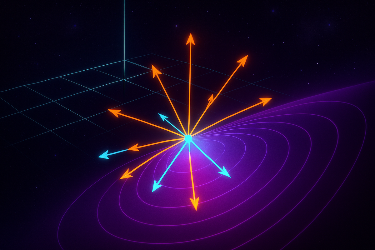
In multivariable calculus, at any point you can move in infinitely many directions. To specify a direction, you use a unit vector u.

A unit vector has length 1: ||u|| = 1. It points in the direction you want to analyze.

In 2D: u = (u₁, u₂) with u₁² + u₂² = 1

In 3D: u = (u₁, u₂, u₃) with u₁² + u₂² + u₃² = 1

For example:

• u = (1, 0) points in the positive x-direction
• u = (0, 1) points in the positive y-direction
• u = (1/√2, 1/√2) points diagonally at 45° between x and y
• u = (3/5, 4/5) points at an angle where the x-component is 3/5 and y-component is 4/5

The key is that u is normalized (length 1), so it represents pure direction without magnitude.

The Definition: Derivative in Direction u

The directional derivative of f at point x in the direction u is denoted D_uf(x) and defined as:

D_uf(x) = lim (h→0) [f(x + hu) - f(x)] / h

This is the familiar derivative limit, but instead of moving along the x-axis by h, you're moving in the direction u by a distance h.

Geometrically: imagine standing at point x on the surface z = f(x, y). You walk in direction u for a small distance h. How much does the height z change per unit distance traveled? That's D_uf.

The directional derivative generalizes partial derivatives:

• D_if = ∂f/∂x (where i = (1, 0, 0) is the unit vector in the x-direction)
• D_jf = ∂f/∂y (where j = (0, 1, 0) is the unit vector in the y-direction)
• D_kf = ∂f/∂z (where k = (0, 0, 1) is the unit vector in the z-direction)

Partial derivatives are just directional derivatives along the coordinate axes.

The Formula: Dot Product with the Gradient

Here's the computationally powerful result: if f is differentiable, then the directional derivative in direction u is:

D_uf(x) = ∇f(x) · u

where · denotes the dot product.

In 2D: D_uf = (∂f/∂x, ∂f/∂y) · (u₁, u₂) = (∂f/∂x)u₁ + (∂f/∂y)u₂

In 3D: D_uf = (∂f/∂x, ∂f/∂y, ∂f/∂z) · (u₁, u₂, u₃) = (∂f/∂x)u₁ + (∂f/∂y)u₂ + (∂f/∂z)u₃

This formula is remarkable: to find the rate of change in any direction, you just take the dot product of the gradient (which you compute once) with the unit vector in that direction.

You don't need to go back to the limit definition for every new direction. Compute the gradient, pick a direction, dot them together, done.

Why the Formula Works: Geometric Insight

The dot product formula D_uf = ∇f · u connects to the geometric meaning of the gradient.

Recall that the dot product of two vectors a · b = ||a|| ||b|| cos(θ), where θ is the angle between them.

Since u is a unit vector (||u|| = 1), we have:

D_uf = ∇f · u = ||∇f|| cos(θ)

where θ is the angle between the gradient and the direction u.

This reveals:

• When θ = 0 (moving parallel to the gradient), cos(θ) = 1, so D_uf = ||∇f||, the maximum possible directional derivative
• When θ = 90° (moving perpendicular to the gradient), cos(θ) = 0, so D_uf = 0—no change in that direction
• When θ = 180° (moving opposite to the gradient), cos(θ) = -1, so D_uf = -||∇f||, the maximum rate of decrease

This proves that the gradient points in the direction of maximum increase, and the rate of increase in that direction is the magnitude of the gradient.

Moving perpendicular to the gradient means moving along a level curve (where f is constant), so the directional derivative is zero.

The dot product formula encodes all of this geometry in one compact expression.

Computing Directional Derivatives: Examples

Example 1: f(x, y) = x² + 2y², find the directional derivative at (1, 1) in the direction u = (3/5, 4/5).

First, compute the gradient: ∇f = (∂f/∂x, ∂f/∂y) = (2x, 4y)

At (1, 1): ∇f(1, 1) = (2, 4)

Now compute the directional derivative: D_uf(1, 1) = ∇f(1, 1) · u = (2, 4) · (3/5, 4/5) = 2(3/5) + 4(4/5) = 6/5 + 16/5 = 22/5

So the function increases at a rate of 22/5 per unit distance when moving from (1, 1) in the direction u.

Example 2: f(x, y, z) = xyz, find D_uf at (2, 1, 3) in the direction of the vector v = (1, 2, 2).

First, normalize v to get a unit vector: ||v|| = √(1² + 2² + 2²) = √9 = 3

So u = v/||v|| = (1/3, 2/3, 2/3)

Compute the gradient: ∇f = (yz, xz, xy)

At (2, 1, 3): ∇f(2, 1, 3) = (1·3, 2·3, 2·1) = (3, 6, 2)

Compute the directional derivative: D_uf(2, 1, 3) = (3, 6, 2) · (1/3, 2/3, 2/3) = 3(1/3) + 6(2/3) + 2(2/3) = 1 + 4 + 4/3 = 19/3

The function increases at rate 19/3 in that direction.

Example 3: For f(x, y) = e^x sin(y), find the direction of maximum increase at (0, π/4).

The direction of maximum increase is the gradient direction.

∇f = (e^x sin(y), e^x cos(y))

At (0, π/4): ∇f(0, π/4) = (e^0 sin(π/4), e^0 cos(π/4)) = (√2/2, √2/2)

This vector points in the direction of maximum increase. To express it as a unit vector: ||∇f|| = √[(√2/2)² + (√2/2)²] = √(1/2 + 1/2) = 1

So the gradient is already a unit vector: u = (√2/2, √2/2), pointing at 45° between the x and y axes.

The maximum rate of increase is ||∇f|| = 1.

Level Curves and Zero Directional Derivative

When you move tangent to a level curve, the directional derivative is zero because f doesn't change along a level curve.

Mathematically: if u is tangent to the level curve f(x, y) = c, then:

D_uf = ∇f · u = 0

This confirms that ∇f is perpendicular to level curves: if the gradient is perpendicular to u, their dot product is zero.

Example: For f(x, y) = x² + y², the level curves are circles x² + y² = r².

At the point (3, 4) on the circle of radius 5, the gradient is ∇f = (2x, 2y) = (6, 8).

A vector tangent to the circle at (3, 4) is u = (-4/5, 3/5) (perpendicular to the radius).

Check: ∇f · u = (6, 8) · (-4/5, 3/5) = 6(-4/5) + 8(3/5) = -24/5 + 24/5 = 0.

The directional derivative is zero, as expected for motion along the level curve.

Maximum and Minimum Rates of Change

The directional derivative D_uf = ||∇f|| cos(θ) depends on the angle θ between u and ∇f.

• Maximum rate of increase: occurs when θ = 0, i.e., u = ∇f / ||∇f||. The maximum rate is ||∇f||.
• Maximum rate of decrease: occurs when θ = 180°, i.e., u = -∇f / ||∇f||. The rate is -||∇f||.
• Zero rate of change: occurs when θ = 90°, i.e., u is perpendicular to ∇f. Moving along a level curve.

This is why ||∇f|| is such an important quantity: it bounds all directional derivatives. You can't change f faster than ||∇f|| in any direction.

Directional Derivatives and Optimization

In optimization, you often want to move in the direction that decreases a function most rapidly (gradient descent) or increases it most rapidly (gradient ascent).

The directional derivative tells you: given a direction, how much will the function change?

If you're constrained to move in certain directions (say, along a path or surface), the directional derivative tells you whether you're going uphill or downhill along that constraint.

Example: Suppose you're climbing a hill (height h(x, y)) but you must follow a road that runs in the direction u = (1/√2, 1/√2). Is the road taking you uphill?

Compute D_uh. If it's positive, you're climbing. If it's negative, you're descending.

This is sensitivity analysis for constrained motion: you can't move freely in any direction, but you can move along allowed paths, and the directional derivative tells you the rate of change along those paths.

Higher-Order Directional Derivatives

Just as you can take second derivatives in single-variable calculus, you can take second directional derivatives.

The second directional derivative in direction u is:

D_u²f = D_u(D_uf)

In terms of the gradient, this gets more complex. For u = (u₁, u₂), you have:

D_u²f = u₁² (∂²f/∂x²) + 2u₁u₂ (∂²f/∂x∂y) + u₂² (∂²f/∂y²)

This is a quadratic form involving the Hessian matrix (the matrix of second partial derivatives).

The second directional derivative measures the curvature of the function in direction u:

• If D_u²f > 0, the function curves upward in that direction (convex)
• If D_u²f < 0, the function curves downward in that direction (concave)
• If D_u²f = 0, the function is locally linear in that direction

This is used in the second derivative test for classifying critical points.

Directional Derivatives in Curvilinear Coordinates

The formula D_uf = ∇f · u works in any coordinate system, provided you compute ∇f correctly in those coordinates.

For example, in polar coordinates (r, θ), the gradient is:

∇f = (∂f/∂r) e_r + (1/r)(∂f/∂θ) e_θ

If you want the directional derivative in the direction u = cos(α) e_r + sin(α) e_θ, you compute:

D_uf = ∇f · u = (∂f/∂r) cos(α) + (1/r)(∂f/∂θ) sin(α)

The key is that u must be a unit vector in the same coordinate basis as ∇f.

When Directional Derivatives Don't Exist

If f isn't differentiable at a point, directional derivatives might not exist, or they might exist in some directions but not others, or they might exist in all directions but not agree with the gradient formula.

Example: f(x, y) = √(|xy|) at the origin.

You can compute directional derivatives along the axes (they're zero), but the gradient doesn't exist because the partial derivatives don't exist at (0, 0).

For nice functions (continuously differentiable), directional derivatives always exist and are given by D_uf = ∇f · u.

For pathological functions, you have to be more careful.

Practical Applications

Computer graphics: Normal vectors to surfaces are gradients of implicit surface functions. Directional derivatives tell you how light intensity varies as you move across a surface.

Fluid dynamics: The directional derivative of velocity in the direction of flow gives the acceleration of a fluid particle (the material derivative).

Thermodynamics: The rate of temperature change as you move through space in a specific direction is a directional derivative of the temperature field.

Economics: If utility u(x, y) depends on consumption of two goods, the directional derivative in the direction u = (1/√2, 1/√2) tells you the rate of utility increase if you increase both goods equally.

Machine learning: When optimizing over a subset of parameters (holding others fixed), you're computing a directional derivative in a restricted subspace.

In every case, the directional derivative answers: "If I move this way, how does the quantity change?"

The Conceptual Core: Projecting Change

The formula D_uf = ∇f · u has a beautiful interpretation: the directional derivative is the projection of the gradient onto the direction u.

The gradient ∇f encodes all directional information about how f changes. To extract the rate of change in a specific direction, you project ∇f onto that direction via the dot product.

This is why the gradient is so fundamental: it's the universal object that contains all directional derivatives. Every directional derivative is just a component of the gradient in the relevant direction.

This is the multivariable analogue of how the derivative f'(x) tells you the rate of change as x increases. In multiple variables, "the rate of change" depends on direction, so you need a vector (the gradient) to capture all possible rates, and you extract specific rates via projection (dot product with u).

Connecting to the Chain Rule

The directional derivative is intimately connected to the chain rule.

If you move along a path r(t) = (x(t), y(t), z(t)) in space, the rate of change of f along the path is:

df/dt = ∇f · dr/dt

where dr/dt is the velocity vector of the path.

This is a directional derivative in the direction of motion (after normalizing for speed).

The chain rule for multivariable functions generalizes this: derivatives propagate via dot products with gradients.

We'll explore this in detail in the next article on the multivariable chain rule.

What's Next

You now have the full picture of differentiation in multiple variables:

• Partial derivatives measure change along coordinate axes
• The gradient packages partial derivatives into a vector pointing uphill
• Directional derivatives measure change in any direction via ∇f · u

Next, we tackle the multivariable chain rule, which describes how derivatives compose when you have functions of functions.

This is where things get network-like: when one variable depends on others, which depend on still others, how do you track how changes propagate through the dependency graph?

The answer involves gradients, directional derivatives, and the Jacobian matrix—a generalization of the derivative to vector-valued functions.

After that, we'll shift from differentiation to integration: how to accumulate quantities over regions (double integrals), volumes (triple integrals), and how to transform between coordinate systems (Jacobians again, but for integrals).

The directional derivative completes the differentiation toolkit. Now we're ready to see how these tools compose and integrate into the full machinery of multivariable calculus.

Let's keep building.

Part 4 of the Multivariable Calculus series.

Previous: The Gradient: All Partial Derivatives in One Vector Next: The Chain Rule in Multiple Variables