Double Integrals: Integrating Over Regions

Single-variable integration computes area under a curve. Double integration? That computes volume under a surface, or mass over a region, or total heat energy in a plate—any quantity that accumulates continuously across a two-dimensional domain.

This is where calculus becomes genuinely spatial. You're not summing along a line anymore. You're summing over a region—a rectangle, a disk, an irregular blob—slicing it into infinitesimal pieces and adding up their contributions.

Double integrals are the foundation of computing area, volume, mass, center of mass, probability over regions, flux through surfaces—anywhere you need to aggregate a quantity distributed across a 2D space.

The Setup: Integrating Over a Region

In single-variable calculus, ∫_a^b f(x)dx integrates f from x = a to x = b.

In multivariable calculus, you integrate over a region R in the xy-plane:

∬_R f(x, y) dA

where dA is an infinitesimal area element.

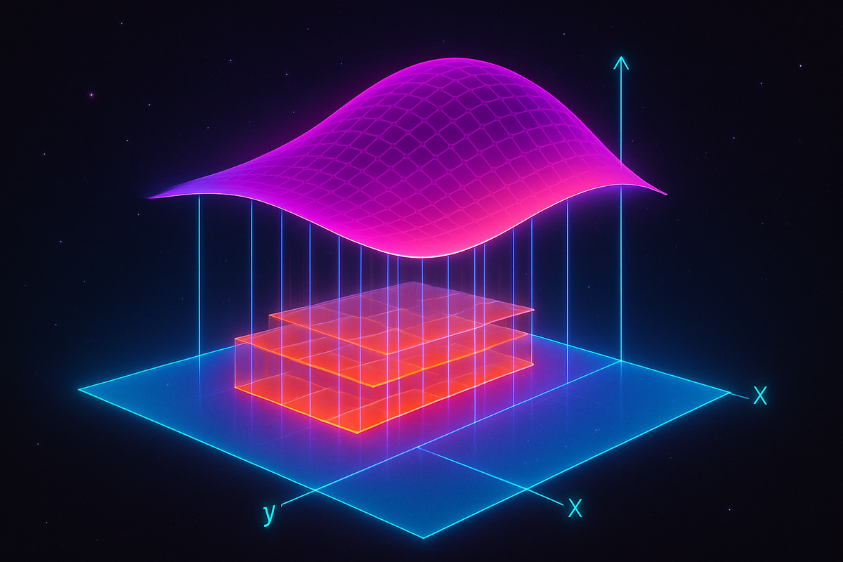
Geometrically, if f(x, y) ≥ 0, this integral equals the volume of the solid region bounded by:

• The surface z = f(x, y) above
• The region R in the xy-plane below

If f(x, y) can be negative, the integral gives signed volume (positive where f > 0, negative where f < 0).

If f represents density, the integral gives total mass. If f is temperature, the integral gives total thermal energy. The interpretation depends on the physical meaning of f, but the mathematical operation is the same: sum f(x, y) over all infinitesimal area elements in R.

Computing Double Integrals: Iterated Integration

The key insight: a double integral over a region can be computed as two nested single-variable integrals.

This is Fubini's theorem: under reasonable conditions (f continuous, R is a nice region), you can write:

∬_R f(x, y) dA = ∫a^b ∫{g₁(x)}^{g₂(x)} f(x, y) dy dx

or equivalently:

∬_R f(x, y) dA = ∫c^d ∫{h₁(y)}^{h₂(y)} f(x, y) dx dy

The order matters: you choose whether to integrate with respect to y first (inner integral) and then x (outer integral), or vice versa.

How to set limits:

• For dy dx order: the outer integral's limits are the x-range of the region (say, a to b). For each fixed x, the inner integral's limits are the y-range at that x-value (from y = g₁(x) to y = g₂(x), where g₁ and g₂ bound the region).
• For dx dy order: the outer integral's limits are the y-range (say, c to d). For each fixed y, the inner integral's limits are the x-range at that y-value (from x = h₁(y) to x = h₂(y)).

Example 1: Rectangular region

Let R be the rectangle [0, 2] × [0, 3] (0 ≤ x ≤ 2, 0 ≤ y ≤ 3).

Compute ∬_R (x² + y) dA.

Using dy dx order:

∬_R (x² + y) dA = ∫₀² ∫₀³ (x² + y) dy dx

Inner integral (integrate with respect to y, treating x as constant):

∫₀³ (x² + y) dy = [x²y + y²/2]₀³ = 3x² + 9/2

Outer integral:

∫₀² (3x² + 9/2) dx = [x³ + (9/2)x]₀² = 8 + 9 = 17

So ∬_R (x² + y) dA = 17.

Example 2: Non-rectangular region

Let R be the triangular region bounded by x = 0, y = 0, and x + y = 1.

This is the triangle with vertices (0, 0), (1, 0), (0, 1).

For a given x in [0, 1], y ranges from 0 to 1 - x.

Compute ∬_R xy dA.

∬_R xy dA = ∫₀¹ ∫₀^{1-x} xy dy dx

Inner integral:

∫₀^{1-x} xy dy = x[y²/2]₀^{1-x} = x(1-x)²/2

Outer integral:

∫₀¹ x(1-x)²/2 dx = (1/2) ∫₀¹ x(1 - 2x + x²) dx = (1/2) ∫₀¹ (x - 2x² + x³) dx

= (1/2)[x²/2 - 2x³/3 + x⁴/4]₀¹ = (1/2)(1/2 - 2/3 + 1/4) = (1/2)(6/12 - 8/12 + 3/12) = (1/2)(1/12) = 1/24

So ∬_R xy dA = 1/24.

Changing the Order of Integration

Sometimes one order of integration is easier than the other.

For the triangular region above, we integrated with dy dx order. Could we use dx dy?

Yes. For a given y in [0, 1], x ranges from 0 to 1 - y.

∬_R xy dA = ∫₀¹ ∫₀^{1-y} xy dx dy

Inner integral:

∫₀^{1-y} xy dx = y[x²/2]₀^{1-y} = y(1-y)²/2

Outer integral:

∫₀¹ y(1-y)²/2 dy = (1/2) ∫₀¹ y(1 - 2y + y²) dy = (1/2) ∫₀¹ (y - 2y² + y³) dy

= (1/2)[y²/2 - 2y³/3 + y⁴/4]₀¹ = 1/24

Same answer, as it must be by Fubini's theorem.

But sometimes one order leads to integrals you can't compute analytically, while the other works. Choosing the right order is part of the art of integration.

The Geometric Meaning: Volume Under a Surface

If f(x, y) ≥ 0, then ∬_R f(x, y) dA is the volume of the solid under the surface z = f(x, y) and above the region R.

Example: f(x, y) = 4 - x² - y² over the disk x² + y² ≤ 1.

This is a paraboloid, and the region is a circular disk of radius 1.

The double integral ∬_R (4 - x² - y²) dA computes the volume under the paraboloid and above the disk.

In Cartesian coordinates, the limits for the disk are messy. For a given x in [-1, 1], y ranges from -√(1-x²) to √(1-x²).

∬R (4 - x² - y²) dA = ∫{-1}^1 ∫_{-√(1-x²)}^{√(1-x²)} (4 - x² - y²) dy dx

This is doable but tedious. Polar coordinates make it trivial (we'll revisit this when discussing coordinate changes).

Area of a Region

If you set f(x, y) = 1, the double integral computes the area of the region R:

Area(R) = ∬_R 1 dA

This is a special case where the "height" of the solid is uniformly 1, so the volume equals the base area.

Example: Find the area of the ellipse x²/a² + y²/b² ≤ 1.

Area = ∬_R 1 dA

In Cartesian coordinates, for a given x in [-a, a], y ranges from -b√(1 - x²/a²) to b√(1 - x²/a²).

Area = ∫{-a}^a ∫{-b√(1-x²/a²)}^{b√(1-x²/a²)} 1 dy dx

= ∫_{-a}^a 2b√(1 - x²/a²) dx

Substitute u = x/a, dx = a du:

= 2b ∫{-1}^1 a√(1 - u²) du = 2ab ∫{-1}^1 √(1 - u²) du

The integral ∫_{-1}^1 √(1 - u²) du is the area of a semicircle of radius 1, which is π(1)²/2 = π/2. But we have the full circle (from -1 to 1), so it's π.

Wait, let's recalculate: ∫_{-1}^1 √(1 - u²) du is the area under a semicircle from -1 to 1, which is the full circle's area divided by 2 (since the semicircle is the top half). Actually, the area of a circle of radius 1 is π, and the area under the curve √(1 - u²) from -1 to 1 is half the circle's area, so π/2.

Hmm, let me reconsider. The function √(1 - u²) traces the upper semicircle of radius 1. The integral ∫_{-1}^1 √(1 - u²) du is the area under that semicircle, which is indeed half the circle: π(1)²/2 = π/2.

So Area = 2ab · (π/2) = πab.

That's the correct formula for the area of an ellipse with semi-axes a and b.

Double integrals can compute areas of non-standard regions by integrating 1 over them.

Double Integrals for Mass and Density

If ρ(x, y) is the density (mass per unit area) at point (x, y), then the total mass of a region R is:

M = ∬_R ρ(x, y) dA

Example: A thin plate occupies the region 0 ≤ x ≤ 1, 0 ≤ y ≤ 1, with density ρ(x, y) = x + y.

Total mass:

M = ∬_R (x + y) dA = ∫₀¹ ∫₀¹ (x + y) dy dx

Inner integral:

∫₀¹ (x + y) dy = [xy + y²/2]₀¹ = x + 1/2

Outer integral:

∫₀¹ (x + 1/2) dx = [x²/2 + x/2]₀¹ = 1/2 + 1/2 = 1

Total mass is 1 (in whatever units).

This generalizes: double integrals let you compute total quantities (mass, charge, heat) from density functions.

Center of Mass

The center of mass (x̄, ȳ) of a region R with density ρ(x, y) is:

x̄ = (1/M) ∬_R x ρ(x, y) dA

ȳ = (1/M) ∬_R y ρ(x, y) dA

where M = ∬_R ρ(x, y) dA is the total mass.

These are weighted averages: x̄ is the average x-coordinate, weighted by density.

Example: For the plate above with ρ(x, y) = x + y on [0, 1] × [0, 1], we found M = 1.

Compute x̄:

x̄ = ∬_R x(x + y) dA = ∫₀¹ ∫₀¹ (x² + xy) dy dx

Inner integral:

∫₀¹ (x² + xy) dy = [x²y + xy²/2]₀¹ = x² + x/2

Outer integral:

∫₀¹ (x² + x/2) dx = [x³/3 + x²/4]₀¹ = 1/3 + 1/4 = 7/12

So x̄ = 7/12.

By symmetry (ρ(x, y) = x + y is symmetric under swapping x and y), ȳ = 7/12 as well.

The center of mass is (7/12, 7/12), shifted toward the upper-right corner where the density is higher.

Fubini's Theorem and When Order Doesn't Matter

Fubini's theorem says that if f is continuous on a rectangular region (or more generally, integrable), then:

∫_a^b ∫_c^d f(x, y) dy dx = ∫_c^d ∫_a^b f(x, y) dx dy

The order of integration doesn't affect the result.

This holds for non-rectangular regions too, provided the region is "nice" (bounded, piecewise smooth boundary) and f is integrable.

The practical consequence: you can choose whichever order makes the computation easier.

If the inner integral in one order is hard or impossible to compute analytically, try the other order.

Non-Rectangular Regions: Type I and Type II

Regions are often classified by how they're bounded:

Type I (vertically simple): For each x in [a, b], y ranges from g₁(x) to g₂(x).

∬_R f(x, y) dA = ∫a^b ∫{g₁(x)}^{g₂(x)} f(x, y) dy dx

Type II (horizontally simple): For each y in [c, d], x ranges from h₁(y) to h₂(y).

∬_R f(x, y) dA = ∫c^d ∫{h₁(y)}^{h₂(y)} f(x, y) dx dy

Some regions are both Type I and Type II. Some are neither (requiring subdivision into sub-regions).

Example: The region bounded by y = x² and y = 2x.

Find the intersection points: x² = 2x → x² - 2x = 0 → x(x - 2) = 0 → x = 0 or x = 2.

So the region is between the parabola y = x² (below) and the line y = 2x (above), for x in [0, 2].

This is Type I: for each x in [0, 2], y ranges from x² to 2x.

∬R f(x, y) dA = ∫₀² ∫{x²}^{2x} f(x, y) dy dx

Alternatively, express as Type II: for y in [0, 4], x ranges from y/2 (from the line y = 2x) to √y (from the parabola y = x²).

∬R f(x, y) dA = ∫₀⁴ ∫{y/2}^{√y} f(x, y) dx dy

Both descriptions are valid; choose based on which integrals are easier.

When to Use Which Order

Use dy dx if:

• The region is naturally described as "for each x, y ranges from ... to ..."
• The inner integral ∫ f(x, y) dy is easy to compute

Use dx dy if:

• The region is naturally described as "for each y, x ranges from ... to ..."
• The inner integral ∫ f(x, y) dx is easy to compute

Example where order matters: ∬_R e^(y²) dA over the triangle with vertices (0, 0), (1, 0), (1, 1).

If you try dy dx order:

∫₀¹ ∫₀^x e^(y²) dy dx

The inner integral ∫ e^(y²) dy has no elementary antiderivative. You're stuck.

But try dx dy order:

∫₀¹ ∫_y¹ e^(y²) dx dy

Inner integral (integrating with respect to x, treating y as constant):

∫_y¹ e^(y²) dx = e^(y²)[x]_y¹ = e^(y²)(1 - y)

Outer integral:

∫₀¹ e^(y²)(1 - y) dy

Substitute u = y², du = 2y dy, so (1 - y)dy is trickier. Actually, let's use integration by parts or recognize this is computable.

Alternatively, substitute u = y² for the exponential part and handle (1 - y) separately. This is doable, whereas the dy dx order was impossible.

The moral: always check both orders before giving up.

Polar Coordinates Preview

For regions with circular symmetry (disks, annuli, sectors), Cartesian coordinates lead to messy limits involving square roots.

Polar coordinates (r, θ) simplify these integrals drastically.

In polar coordinates, the area element dA becomes r dr dθ (not just dr dθ—the r factor accounts for how area elements get larger as you move away from the origin).

We'll explore this in detail in the Jacobian article, but here's a preview:

For a disk of radius R:

∬_{x² + y² ≤ R²} f(x, y) dA = ∫₀^{2π} ∫₀^R f(r cos θ, r sin θ) r dr dθ

The r factor is crucial—it's part of the Jacobian of the coordinate transformation.

The Conceptual Core: Summing Over a Region

The single-variable integral ∫_a^b f(x) dx sums f along an interval.

The double integral ∬_R f(x, y) dA sums f over a region.

The notation dA (or sometimes dx dy or dy dx, depending on order) represents an infinitesimal area element.

You partition the region into tiny rectangles of area ΔA, evaluate f at a point in each rectangle, sum f(x, y) ΔA over all rectangles, then take the limit as ΔA → 0.

Fubini's theorem says this can be done as nested one-dimensional sums (integrals).

This is powerful: you reduce a two-dimensional problem to two one-dimensional problems, computed sequentially.

Common Applications

Volume under a surface: ∬_R f(x, y) dA where f(x, y) is height.

Area of a region: ∬_R 1 dA.

Mass of a plate: ∬_R ρ(x, y) dA where ρ is density.

Average value of f over R: (1/Area(R)) ∬_R f(x, y) dA.

Probability: If p(x, y) is a probability density function over R, then ∬_R p(x, y) dA is the probability that (X, Y) lies in R.

Moments of inertia: ∬_R r²(x, y) ρ(x, y) dA where r is distance from an axis.

Every application boils down to: "sum this quantity over this region."

What's Next

Double integrals handle two-dimensional regions. What about three-dimensional volumes?

That's where triple integrals come in: ∭_V f(x, y, z) dV, integrating over a volume V in three-dimensional space.

The mechanics are similar—nested integrals, now three deep—but the geometric intuition shifts from "volume under a surface" to "total quantity throughout a volume."

After triple integrals, we'll tackle the Jacobian and changes of variables, which formalize how to switch from Cartesian to polar (or cylindrical, spherical, etc.) coordinates when integrating.

Then we'll close with Lagrange multipliers for constrained optimization, bringing together gradients and critical points to solve optimization problems with constraints.

Double integrals are the gateway to spatial integration. Once you internalize the setup—choose a region, choose an order, compute nested integrals—the rest is technique.

Let's keep going.

Part 6 of the Multivariable Calculus series.

Previous: The Chain Rule in Multiple Variables Next: Triple Integrals: Integrating Through Volumes