First-Order ODEs: The Simplest Differential Equations

First-Order ODEs: The Simplest Differential Equations | Ideasthesia

First-order ordinary differential equations are the simplest differential equations that aren't trivial. They involve the first derivative and nothing higher.

Standard form: dy/dx = f(x, y)

That's it. The rate of change of y depends on x and possibly y itself, but not on any higher derivatives.

First-order ODEs model basic growth, decay, cooling, mixing—any process where the current rate of change depends only on the current state, not on acceleration or higher-order dynamics.

Why First-Order Matters

First-order equations are the foundation. Before you can handle oscillation (second-order) or complex wave dynamics (higher-order or PDEs), you need to master first-order techniques.

But they're not just pedagogical. First-order ODEs describe real phenomena:

Radioactive decay: dN/dt = -λN (decay rate proportional to current amount)
Newton's cooling: dT/dt = -k(T - T_ambient) (cooling rate proportional to temperature difference)
Population growth: dP/dt = rP (growth rate proportional to population)
Mixing problems: dQ/dt = r_in - r_out (rate of change equals input minus output)
RC circuits: dQ/dt + Q/(RC) = V/R (charge accumulation in capacitor)

Every one of these is first-order. No acceleration, no oscillation—just straightforward evolution based on current state.

General Form

The general first-order ODE:

dy/dx = f(x, y)

The function f can depend on x, on y, or on both.

Examples:

dy/dx = x² (depends only on x—autonomous in y)

dy/dx = y (depends only on y—autonomous in x)

dy/dx = xy (depends on both)

Each requires different solution strategies.

Autonomous vs Non-Autonomous

An equation is autonomous if f doesn't explicitly depend on the independent variable.

Autonomous: dy/dt = y(1 - y) (no explicit t on the right side)

Non-autonomous: dy/dt = ty (explicit t appears)

Autonomous equations have special properties. Solutions are time-invariant—shifting the initial time doesn't change the shape of the solution, only its phase.

They're also easier to analyze qualitatively. You can draw phase portraits and identify equilibria without solving explicitly.

Existence and Uniqueness

Not every differential equation has a solution. Not every solution is unique.

Existence Theorem: If f(x, y) is continuous, solutions exist locally (at least for a small interval around the initial condition).

Uniqueness Theorem: If f(x, y) and ∂f/∂y are both continuous, solutions are unique.

Translation: If the equation is well-behaved (no discontinuities, no weird singularities), you get exactly one solution through each initial condition.

Example where uniqueness fails:

dy/dx = y^(1/2) with y(0) = 0

Two solutions:

y = 0 (constant solution)
y = (x/2)² (nontrivial solution)

Both satisfy the equation and the initial condition. Why? Because ∂f/∂y = 1/(2√y) blows up at y = 0, violating the uniqueness condition.

Generally, you won't encounter non-unique solutions unless you specifically look for pathological cases. But it's good to know the theory.

Solution Methods Overview

First-order ODEs split into categories based on structure:

Separable equations: Can write as g(y)dy = h(x)dx
Linear equations: Form dy/dx + P(x)y = Q(x)
Exact equations: Form M(x,y)dx + N(x,y)dy = 0 where ∂M/∂y = ∂N/∂x
Bernoulli equations: Form dy/dx + P(x)y = Q(x)y^n
Homogeneous equations: Form dy/dx = f(y/x)

Each type has a dedicated technique. We'll cover the major ones in this series.

Direct Integration

The simplest case: dy/dx = f(x) (f depends only on x).

Solution: Integrate both sides.

dy = f(x)dx

y = ∫f(x)dx + C

Example: dy/dx = 3x²

y = ∫3x²dx = x³ + C

Done. This is just antidifferentiation—no special techniques needed.

Separable Equations (Preview)

If you can write the equation as:

dy/dx = g(x)h(y)

(right side factors into function of x times function of y), it's separable.

Rewrite as:

dy/h(y) = g(x)dx

Integrate both sides:

∫dy/h(y) = ∫g(x)dx

Example: dy/dx = xy

dy/y = xdx

ln|y| = (x²/2) + C

y = Ae^(x²/2) (where A = ±e^C)

We'll dive deep into separable equations in the next article.

Linear First-Order Equations (Preview)

Standard form: dy/dx + P(x)y = Q(x)

These require the integrating factor method:

Multiply by μ(x) = e^(∫P(x)dx) to make the left side a perfect derivative.

The equation becomes:

d/dx[μy] = μQ

Integrate:

μy = ∫μQ dx + C

Solve for y.

Example: dy/dx + y = e^x

Here P(x) = 1, Q(x) = e^x.

Integrating factor: μ = e^(∫1dx) = e^x

Multiply: e^x(dy/dx) + e^x y = e^(2x)

Left side is d/dx[e^x y], so:

e^x y = ∫e^(2x)dx = (1/2)e^(2x) + C

y = (1/2)e^x + Ce^(-x)

We'll explore this fully in the linear equations article.

Qualitative Analysis

Sometimes you don't need an exact solution. You just need to understand behavior.

Phase line analysis: For autonomous equations dy/dt = f(y), plot f(y) vs y.

Where f(y) = 0: equilibrium points (y doesn't change)
Where f(y) > 0: y increases
Where f(y) < 0: y decreases

This tells you long-term behavior without solving.

Example: dy/dt = y(1 - y) (logistic equation)

Equilibria: y = 0 and y = 1

For 0 < y < 1: dy/dt > 0 (y increases toward 1)
For y > 1: dy/dt < 0 (y decreases toward 1)
y = 0 is unstable (solutions move away)
y = 1 is stable (solutions approach it)

Phase line:

y = 1  ← stable equilibrium
 ↑
y = 0  ← unstable equilibrium

Without solving, you know: starting above 0, the solution approaches 1 asymptotically.

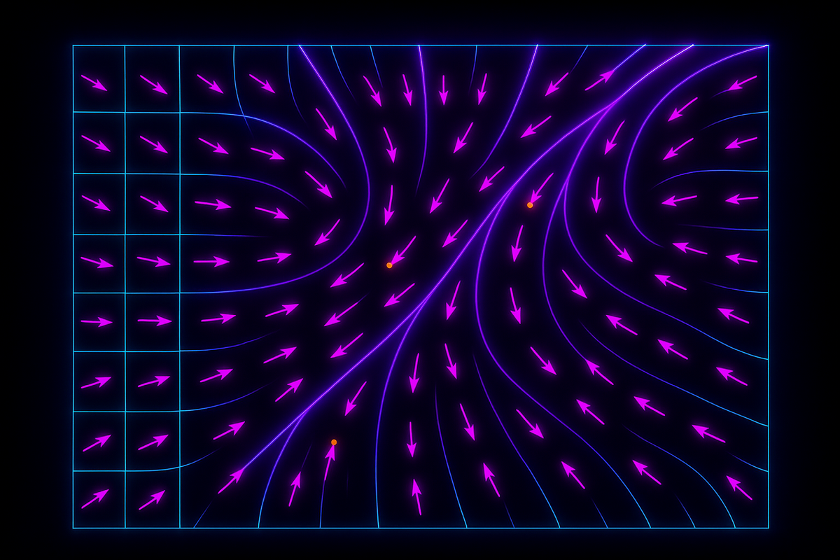
Slope Fields

Another qualitative tool: slope fields (or direction fields).

At each point (x, y), plot a small line segment with slope f(x, y). This shows the direction of solutions passing through that point.

For dy/dx = x - y:

At (0, 0): slope = 0 (horizontal)
At (1, 0): slope = 1 (diagonal)
At (0, 1): slope = -1 (diagonal down)

Plot these across a grid. Solutions are curves tangent to the field everywhere.

Slope fields give geometric intuition. You see how solutions flow without computing them.

Equilibrium Solutions

An equilibrium (or stationary) solution satisfies dy/dx = 0 everywhere.

For dy/dx = f(x, y), equilibria occur where f(x, y) = 0.

Example: dy/dx = y² - 1

Equilibria: y² = 1, so y = 1 and y = -1.

These are constant solutions. Once the system reaches y = 1 or y = -1, it stays there forever.

Stability:

Stable: Nearby solutions approach the equilibrium
Unstable: Nearby solutions diverge away
Semi-stable: Stable from one side, unstable from the other

For y = 1:

If y slightly above 1: dy/dx = (1+ε)² - 1 ≈ 2ε > 0 (y increases further—unstable)
If y slightly below 1: dy/dx = (1-ε)² - 1 ≈ -2ε < 0 (y decreases further—unstable)

Both equilibria are unstable.

Stability analysis tells you long-term behavior without explicit solutions.

Implicit vs Explicit Solutions

Some solutions can't be written as y = f(x). They're implicit: some relation F(x, y) = 0.

Example: dy/dx = -x/y

Separate: y dy = -x dx

Integrate: y²/2 = -x²/2 + C

Simplify: x² + y² = 2C

This is a circle, not a function. You can't isolate y as a single-valued function of x.

Implicit solutions are valid. They satisfy the differential equation, even if you can't write y = f(x).

Singular Solutions

Sometimes there are solutions that don't fit the general solution family.

Example: Clairaut's equation y = xy' + (y')²

General solution: y = Cx + C² (family of straight lines)

Singular solution: y = -x²/4 (envelope of the lines)

The singular solution satisfies the differential equation but isn't obtainable by choosing C.

These are rare in practice but mathematically interesting.

Numerical Solutions

When analytical methods fail, go numerical.

Euler's method: Starting from (x₀, y₀), step forward:

y_{n+1} = y_n + h·f(x_n, y_n)

where h is the step size.

This approximates the solution by following the slope field in discrete steps.

We'll cover Euler's method in detail later.

Why Master First-Order

First-order ODEs teach you:

How to recognize equation types
How to apply systematic solution techniques
How to interpret solutions physically
How to analyze stability without solving

These skills extend to higher-order equations. Second-order equations reduce to systems of first-order equations. Numerical methods for first-order generalize directly.

Master first-order, and you have the foundation for everything else.

Common First-Order Models

Exponential growth/decay: dy/dt = ky

Solution: y = y₀e^(kt)

Models: population, radioactivity, compound interest.

Logistic growth: dy/dt = ry(1 - y/K)

Solution: y = K/(1 + Ae^(-rt))

Models: population with carrying capacity, epidemic spread.

Newton's cooling: dT/dt = -k(T - T_a)

Solution: T = T_a + (T₀ - T_a)e^(-kt)

Models: cooling objects, temperature equilibration.

Mixing problem: dQ/dt = r_in·c_in - r_out·(Q/V)

Models: salt concentration in tanks, pollutant levels.

Each of these is first-order. Each appears throughout science and engineering.

The Toolkit So Far

For first-order ODEs, you have:

Direct integration (if dy/dx = f(x))
Separation of variables (next article)
Integrating factor (for linear equations)
Qualitative analysis (phase lines, slope fields)
Numerical approximation (Euler's method)

Different equations need different tools. Recognizing which tool applies is half the battle.

Next up: separable differential equations, the most widely applicable first-order technique.

Part 3 of the Differential Equations series.

Previous: Ordinary vs Partial: ODEs and PDEs Next: Separable Equations: When Variables Can Be Pulled Apart