The Gradient: All Partial Derivatives in One Vector

The Gradient: All Partial Derivatives in One Vector | Ideasthesia

The gradient is the multivariable calculus equivalent of the derivative—but it's not a number. It's a vector that points in the direction where the function increases most rapidly, with magnitude equal to the rate of that increase.

This is geometric thinking elevated to computational power. The gradient doesn't just tell you how fast something is changing—it tells you which direction to move to make it change fastest.

In optimization, machine learning, physics, and differential geometry, the gradient is the fundamental object. Understanding it means understanding how multidimensional systems respond to perturbations, how to navigate toward maxima or minima, how fields exert forces.

The Definition: A Vector of Partial Derivatives

For a function f(x, y), the gradient is the vector:

∇f = (∂f/∂x, ∂f/∂y)

For three variables f(x, y, z), it's:

∇f = (∂f/∂x, ∂f/∂y, ∂f/∂z)

The symbol ∇ is called "nabla" or "del." When applied to a scalar function f, it produces the gradient vector ∇f.

In component notation: ∇f = fₓ i + f_y j + f_z k

where i, j, k are the standard unit vectors pointing along the x, y, z axes.

The gradient is constructed from partial derivatives, but it's more than just a list of numbers—it's a geometric object living in the same space as the input variables, with direction and magnitude that encode the local behavior of f.

The Geometry: Direction of Steepest Ascent

Here's the big conceptual payoff: the gradient vector points in the direction of steepest ascent of the function.

Imagine you're standing on a hillside where height is given by z = f(x, y). If you want to climb the hill as steeply as possible, which direction should you walk?

Compute the gradient ∇f at your current position. That vector points directly uphill—the direction where altitude increases most rapidly. The magnitude ||∇f|| tells you how steep the ascent is in that direction.

Conversely, -∇f points in the direction of steepest descent—straight downhill.

This isn't obvious from the definition. Why should packaging partial derivatives into a vector tell you the steepest direction? The proof requires showing that the directional derivative (rate of change in an arbitrary direction) is maximized when you move parallel to ∇f. We'll get to that in the next article.

For now, internalize the geometric picture: the gradient is an arrow at each point, pointing toward increasing values of the function, with length proportional to how rapidly the function increases.

Computing Gradients: Straightforward

Let's compute some gradients to build intuition.

Example 1: f(x, y) = x² + y²

This is a paraboloid—a bowl-shaped surface centered at the origin.

∂f/∂x = 2x ∂f/∂y = 2y

So ∇f = (2x, 2y) = 2(x, y)

Notice: the gradient at any point (x, y) is proportional to the position vector from the origin. It points radially outward, directly away from the center of the bowl. That makes geometric sense—moving outward from the center increases the height most rapidly.

At the origin, ∇f = (0, 0)—the zero vector. This signals a critical point, where the function is at a local minimum.

Example 2: f(x, y, z) = x²y + yz² - xz

∂f/∂x = 2xy - z ∂f/∂y = x² + z² ∂f/∂z = 2yz - x

So ∇f = (2xy - z, x² + z², 2yz - x)

This gradient varies across space in a more complex way, encoding how the function's landscape tilts at each point in 3D.

Example 3: f(x, y) = sin(x) cos(y)

∂f/∂x = cos(x) cos(y) ∂f/∂y = -sin(x) sin(y)

∇f = (cos(x) cos(y), -sin(x) sin(y))

The gradient field here is periodic, with directions and magnitudes oscillating across the xy-plane. At points where sin(x) = 0 or cos(y) = 0, components of the gradient vanish, indicating ridges, valleys, or saddle points.

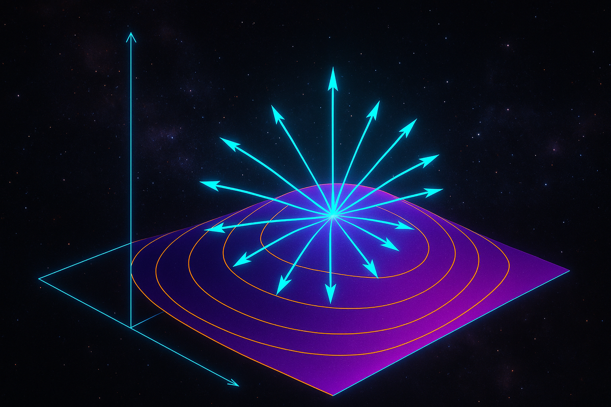
Level Curves and Orthogonality

Here's a beautiful geometric fact: the gradient is perpendicular to level curves (or level surfaces in higher dimensions).

A level curve is the set of points where f(x, y) = c for some constant c. On a topographic map, these are the contour lines of constant elevation.

The gradient ∇f at any point is perpendicular to the level curve passing through that point.

Why? Because moving along a level curve means f stays constant—you're not going uphill or downhill, you're traversing the slope horizontally. The gradient, which points in the direction of maximum increase, must therefore be perpendicular to the curve of no increase.

Example: For f(x, y) = x² + y², the level curves are circles x² + y² = r².

The gradient ∇f = (2x, 2y) points radially outward from the origin, perpendicular to the circular level curves.

This orthogonality property is how you construct normal vectors to surfaces in 3D: if a surface is defined implicitly by f(x, y, z) = 0, then ∇f is perpendicular to the surface, i.e., it's a normal vector.

This is foundational in computer graphics (for lighting calculations), differential geometry (for defining curvature), and physics (for boundary conditions).

Gradient Descent: Following the Gradient Downhill

If you want to find a local minimum of f, you can follow the negative gradient -∇f.

Start at an initial point x₀. Compute the gradient ∇f(x₀). Take a small step in the direction -∇f(x₀):

x₁ = x₀ - α ∇f(x₀)

where α > 0 is the step size (also called learning rate).

Repeat: compute ∇f(x₁), step to x₂ = x₁ - α ∇f(x₁), and so on.

This is gradient descent, the workhorse algorithm of machine learning. When training a neural network, the loss function f depends on millions of parameters. You can't visualize it or solve for the minimum analytically. But you can compute the gradient (via backpropagation) and iteratively step downhill.

The gradient tells you the direction to move. The magnitude ||∇f|| tells you how steep the descent is—if it's large, you're far from a minimum; if it's small, you're approaching a critical point.

Gradient descent isn't guaranteed to find the global minimum (you might get stuck in a local minimum), but it's a practical, scalable way to optimize functions of many variables.

Magnitude of the Gradient: Steepness

The length of the gradient vector, ||∇f||, measures how steeply the function is increasing in the direction of steepest ascent.

For f(x, y), ||∇f|| = √[(∂f/∂x)² + (∂f/∂y)²]

If ||∇f|| is large, the function is changing rapidly—the surface is steep. If ||∇f|| is small, the function is nearly flat.

Where ||∇f|| = 0, the function has a critical point—possibly a local maximum, local minimum, or saddle point. All partial derivatives are zero, meaning there's no slope in any coordinate direction.

Example: For f(x, y) = x² + y², we have ∇f = (2x, 2y), so:

||∇f|| = √[(2x)² + (2y)²] = 2√(x² + y²) = 2r

where r is the distance from the origin. The magnitude of the gradient increases linearly with distance from the center, reflecting the increasing steepness of the paraboloid as you move outward.

Gradients in Different Coordinate Systems

The formula ∇f = (∂f/∂x, ∂f/∂y) assumes Cartesian coordinates. In other coordinate systems, the expression for the gradient looks different.

In polar coordinates (r, θ):

∇f = (∂f/∂r) e_r + (1/r)(∂f/∂θ) e_θ

where e_r and e_θ are unit vectors in the radial and angular directions.

Note the 1/r factor for the angular component—this accounts for the fact that angular displacement corresponds to different arc lengths depending on how far you are from the origin.

In cylindrical coordinates (r, θ, z):

∇f = (∂f/∂r) e_r + (1/r)(∂f/∂θ) e_θ + (∂f/∂z) e_z

In spherical coordinates (ρ, θ, φ):

∇f = (∂f/∂ρ) e_ρ + (1/ρ)(∂f/∂θ) e_θ + (1/(ρ sin θ))(∂f/∂φ) e_φ

The gradient is a geometric object—it's a vector field that doesn't depend on your choice of coordinates. But the formula for computing it does depend on coordinates, because partial derivatives are coordinate-dependent.

This is a recurring theme in differential geometry: geometric objects (gradients, curvature, etc.) are invariant, but their computational expressions depend on the coordinate system.

Gradient Fields: Visualizing Vector Functions

When you compute ∇f at every point in space, you get a vector field—an assignment of a vector to each point.

Visualizing gradient fields reveals the structure of the function's landscape:

Vectors point away from local minima
Vectors point toward local maxima
Vectors circulate around saddle points
Where vectors are dense and long, the function changes rapidly
Where vectors are sparse and short, the function is nearly flat

Example: For f(x, y) = x² - y² (a saddle function), the gradient is ∇f = (2x, -2y).

At points with positive x, the vectors point in the +x direction. At points with positive y, the vectors point in the -y direction. Near the origin, vectors radiate outward along the x-axis and inward along the y-axis—characteristic of a saddle point.

Plotting gradient fields is how you visualize multivariable optimization problems: you're looking for where the field has zero vectors (critical points) and analyzing the flow pattern to determine whether they're maxima, minima, or saddles.

The Gradient and Differentiability

In single-variable calculus, a function is differentiable at a point if the derivative exists there.

In multivariable calculus, existence of all partial derivatives is not enough for differentiability. You need the function to be locally well-approximated by a linear function (technically, its tangent plane).

If f is differentiable at a point, then the gradient ∇f exists there, and the function can be approximated as:

f(x + h) ≈ f(x) + ∇f(x) · h

where h is a small displacement vector and · denotes dot product.

This is the multivariable analogue of f(x + h) ≈ f(x) + f'(x)h from single-variable calculus. The gradient plays the role of the derivative, and the dot product replaces scalar multiplication.

This linear approximation is the foundation of the multivariable chain rule, differentials, and Taylor series in higher dimensions.

Practical Applications

Physics: In electrostatics, the electric field E is the negative gradient of the electric potential V: E = -∇V. The field points in the direction of maximum potential decrease—the direction a positive charge would be pushed.

Thermodynamics: Heat flows in the direction of the negative temperature gradient: -∇T. Heat moves from hot to cold, and the gradient tells you which direction that is.

Economics: In consumer theory, the gradient of the utility function gives the marginal utilities—how much additional utility you get from small increases in each good. Setting it proportional to the price vector gives the optimality condition for utility maximization.

Image processing: Edge detection algorithms compute the gradient of pixel intensity. Large ||∇I|| indicates a sharp change in brightness—an edge.

Fluid dynamics: The pressure gradient ∇p drives fluid flow. Fluids accelerate in the direction of decreasing pressure.

In every case, the gradient captures the idea: "which direction should I move to increase (or decrease) this quantity most effectively?"

Critical Points and Optimization

A critical point of f is a point where ∇f = 0 (the zero vector).

At a critical point, all partial derivatives vanish: ∂f/∂x = 0, ∂f/∂y = 0, ∂f/∂z = 0, ...

This means there's no first-order change in any direction—the function is locally flat.

Critical points are candidates for local maxima and minima. But not every critical point is an extremum:

Local minimum: f is smallest in a neighborhood around the point (like the bottom of a bowl)
Local maximum: f is largest in a neighborhood around the point (like the top of a hill)
Saddle point: f increases in some directions and decreases in others (like a mountain pass)

To distinguish these, you need the second derivative test, which examines the Hessian matrix (the matrix of second partial derivatives). But finding critical points is the first step, and that means solving ∇f = 0.

Example: f(x, y) = x² - y²

∇f = (2x, -2y)

Setting ∇f = (0, 0) gives 2x = 0 and -2y = 0, so the only critical point is (0, 0).

But is it a maximum, minimum, or saddle? Look at the second derivatives:

∂²f/∂x² = 2 (positive, indicating curvature upward in the x-direction)
∂²f/∂y² = -2 (negative, indicating curvature downward in the y-direction)

The function curves up in one direction and down in another—it's a saddle point, not an extremum.

Gradients in Machine Learning

In machine learning, you're often optimizing a loss function L(θ₁, θ₂, ..., θₙ) where the θᵢ are model parameters (weights in a neural network, coefficients in a regression, etc.).

The gradient ∇L tells you how to adjust the parameters to decrease the loss:

If ∂L/∂θᵢ > 0, decreasing θᵢ reduces the loss
If ∂L/∂θᵢ < 0, increasing θᵢ reduces the loss
The magnitude |∂L/∂θᵢ| tells you how sensitive the loss is to that parameter

Gradient descent updates the parameters by stepping in the direction -∇L:

θ ← θ - α ∇L(θ)

For deep neural networks, computing ∇L is nontrivial—it requires backpropagation, an efficient algorithm for computing gradients of compositions (which we'll touch on in the chain rule article).

But the conceptual core is simple: follow the gradient to find the direction of improvement.

Variants like stochastic gradient descent, Adam, RMSprop all involve computing gradients and using them to navigate parameter space toward lower loss.

The gradient is the engine of modern AI.

When the Gradient Doesn't Exist

The gradient exists at a point if all partial derivatives exist there and the function is differentiable.

The gradient doesn't exist:

At discontinuities (obvious)
At corners or cusps (partial derivatives don't exist)
Where partial derivatives exist but the function isn't differentiable (rare for nice functions, but possible)

Example: f(x, y) = |x| + |y| has a corner at the origin. The partial derivatives don't exist there, so neither does the gradient.

For optimization, this matters: you can't use gradient descent through points where the gradient is undefined. You need subgradient methods or other techniques.

The Gradient as a Covector (Advanced)

In differential geometry, the gradient is technically a covector (a one-form), not a vector. This distinction matters when dealing with general coordinate systems and curved spaces.

The partial derivatives ∂f/∂xⁱ transform as covector components. To convert them into a vector (with components that transform correctly), you need a metric—a way of measuring distances and angles.

In Euclidean space with Cartesian coordinates, the metric is trivial (the identity), so the distinction collapses: covectors and vectors look the same.

But in curvilinear coordinates or on curved manifolds, the gradient vector ∇f is related to the covector df by the metric tensor g:

∇f = g⁻¹(df)

This is why the formula for the gradient in polar or spherical coordinates has those 1/r factors—they arise from converting the covector (partial derivatives) into a vector using the metric.

For most applications, you can ignore this and just compute ∇f = (∂f/∂x, ∂f/∂y, ∂f/∂z) in Cartesian coordinates. But it's worth knowing that there's deeper structure here, connecting calculus to geometry.

The Conceptual Core: Local Information, Global Direction

The gradient is a local object—it's computed at a point using derivatives at that point. But it encodes global navigation information: the direction to move to increase the function.

This is the power of calculus: local infinitesimal analysis (derivatives) yields actionable guidance for finite motion (follow the gradient).

In optimization, you don't need to see the whole landscape. You just need to compute the gradient where you are and step in the right direction. Iteratively, this local information guides you to global structure (minima, maxima).

In physics, forces are often gradients of potential energy. The local gradient tells a particle which direction to accelerate—no global knowledge required.

The gradient is how you turn differential calculus into a navigation system.

What's Next

The gradient points in the direction of steepest ascent. But what if you want to know the rate of change in some other direction—not necessarily the steepest one?

That's the directional derivative, which generalizes both partial derivatives (change along coordinate axes) and the gradient (change in the steepest direction).

With directional derivatives, you can analyze how a function changes along any path you choose—curves, diagonals, spirals—using the gradient as the key computational tool.

Then we'll extend to the multivariable chain rule, which describes how gradients propagate through compositions of functions—the mathematical foundation of backpropagation and sensitivity analysis.

The gradient is the linchpin. Everything else in multivariable differentiation builds on it. Once you internalize the gradient as a geometric object—a vector field pointing uphill, encoding both direction and rate—the rest of multivariable calculus becomes navigation through that field.

Let's keep moving.

Part 3 of the Multivariable Calculus series.

Previous: Partial Derivatives: Rates of Change in One Direction Next: Directional Derivatives: Rates of Change in Any Direction