Change of Variables: Jacobians and Coordinate Transforms

When you integrate ∫∫ r dr dθ in polar coordinates instead of ∫∫ dx dy in Cartesian, where does that extra r factor come from?

It's the Jacobian—the scaling factor that accounts for how area (or volume) elements stretch or compress when you change coordinate systems.

This is the mathematical machinery that lets you transform integrals from Cartesian coordinates to polar, cylindrical, spherical, or any other coordinate system. It's why some integrals that are nightmares in Cartesian coordinates become trivial in the right curvilinear system.

The Jacobian is also the key to understanding how derivatives transform under coordinate changes, making it central to differential geometry, physics, and any field where choosing the right coordinates simplifies the problem.

The Problem: Area Elements Change Size

In Cartesian coordinates, a small rectangle with sides dx and dy has area dA = dx dy.

But in polar coordinates (r, θ), the corresponding "rectangle" (a small sector) doesn't have area dr dθ. It has area r dr dθ.

Why? Because as r increases, the same angular increment dθ corresponds to a larger arc length. The area element stretches.

Specifically, at radius r, an angular increment dθ sweeps out an arc of length r dθ. So the area of the sector is (approximately) r dθ times dr, giving dA = r dr dθ.

The Jacobian formalizes this: when you change from (x, y) coordinates to (r, θ) coordinates, the area element transforms as:

dx dy = |J| dr dθ

where J is the Jacobian determinant, and for polar coordinates, |J| = r.

The Jacobian Matrix: Partial Derivatives of the Transformation

Suppose you have a coordinate transformation from (u, v) to (x, y):

• x = x(u, v)
• y = y(u, v)

The Jacobian matrix is the matrix of partial derivatives:

J = [∂x/∂u ∂x/∂v] [∂y/∂u ∂y/∂v]

This matrix describes how small changes in (u, v) map to small changes in (x, y).

The Jacobian determinant (often also called "the Jacobian") is:

det(J) = (∂x/∂u)(∂y/∂v) - (∂x/∂v)(∂y/∂u)

This determinant measures the local area scaling factor: if you have a small region with area ΔA in uv-coordinates, its area in xy-coordinates is approximately |det(J)| ΔA.

Polar Coordinates: The Canonical Example

Polar coordinates relate to Cartesian via:

• x = r cos θ
• y = r sin θ

Compute the Jacobian matrix:

∂x/∂r = cos θ, ∂x/∂θ = -r sin θ ∂y/∂r = sin θ, ∂y/∂θ = r cos θ

J = [cos θ -r sin θ] [sin θ r cos θ]

Jacobian determinant:

det(J) = (cos θ)(r cos θ) - (-r sin θ)(sin θ) = r cos²θ + r sin²θ = r

So |det(J)| = r (assuming r ≥ 0).

The change of variables formula for integrals says:

∬R f(x, y) dx dy = ∬{R'} f(r cos θ, r sin θ) |det(J)| dr dθ = ∬_{R'} f(r cos θ, r sin θ) r dr dθ

That's where the extra r comes from in polar integrals.

Change of Variables Formula: The General Statement

For a double integral, if you transform from (x, y) to (u, v) via x = x(u, v), y = y(u, v), then:

∬R f(x, y) dx dy = ∬{R'} f(x(u,v), y(u,v)) |det(J)| du dv

where R' is the region in uv-coordinates corresponding to R in xy-coordinates, and J is the Jacobian matrix of the transformation.

The absolute value |det(J)| ensures the area element is positive (determinant can be negative if the transformation reverses orientation).

This is the multivariable substitution rule, generalizing u-substitution from single-variable calculus.

Example: Integrating Over an Ellipse

Compute ∬_R (x²/a² + y²/b²) dx dy where R is the ellipse x²/a² + y²/b² ≤ 1.

In Cartesian coordinates, the limits are messy. Transform using:

• x = au
• y = bv

Then the ellipse becomes u² + v² ≤ 1, a unit circle in uv-coordinates.

Jacobian matrix:

J = [∂x/∂u ∂x/∂v] [a 0] [∂y/∂u ∂y/∂v] = [0 b]

det(J) = ab

The integral becomes:

∬R (x²/a² + y²/b²) dx dy = ∬{u²+v²≤1} (u² + v²) ab du dv

Now use polar coordinates for the circle: u = ρ cos φ, v = ρ sin φ, with Jacobian ρ:

= ∫₀^{2π} ∫₀¹ (ρ²) ab ρ dρ dφ = ab ∫₀^{2π} dφ ∫₀¹ ρ³ dρ

= ab · 2π · [ρ⁴/4]₀¹ = ab · 2π · (1/4) = πab/2

By choosing the right coordinates, a complex integral becomes straightforward.

Cylindrical Coordinates

Cylindrical coordinates (r, θ, z) relate to Cartesian (x, y, z) via:

• x = r cos θ
• y = r sin θ
• z = z

The Jacobian matrix is 3×3:

J = [∂x/∂r ∂x/∂θ ∂x/∂z] [cos θ -r sin θ 0] [∂y/∂r ∂y/∂θ ∂y/∂z] = [sin θ r cos θ 0] [∂z/∂r ∂z/∂θ ∂z/∂z] [0 0 1]

Jacobian determinant:

det(J) = 1 · [(cos θ)(r cos θ) - (-r sin θ)(sin θ)] = r(cos²θ + sin²θ) = r

So the volume element in cylindrical coordinates is:

dV = r dr dθ dz

This makes integrals over cylinders, cones, and other rotationally symmetric solids much easier.

Example: Volume of a cylinder of radius R and height h.

In cylindrical coordinates: 0 ≤ r ≤ R, 0 ≤ θ ≤ 2π, 0 ≤ z ≤ h.

Volume = ∫₀^{2π} ∫₀^h ∫₀^R r dr dz dθ = 2π · h · [r²/2]₀^R = 2π · h · R²/2 = πR²h

The standard formula, obtained trivially.

Spherical Coordinates

Spherical coordinates (ρ, θ, φ) relate to Cartesian via:

• x = ρ sin φ cos θ
• y = ρ sin φ sin θ
• z = ρ cos φ

where ρ is the radial distance, θ is the azimuthal angle (same as in cylindrical), and φ is the polar angle (measured from the positive z-axis).

The Jacobian computation is tedious but standard:

det(J) = ρ² sin φ

So the volume element in spherical coordinates is:

dV = ρ² sin φ dρ dθ dφ

This makes integrals over spheres, cones, and spherically symmetric regions straightforward.

Example: Volume of a sphere of radius R.

In spherical coordinates: 0 ≤ ρ ≤ R, 0 ≤ θ ≤ 2π, 0 ≤ φ ≤ π.

Volume = ∫₀^{2π} ∫₀^π ∫₀^R ρ² sin φ dρ dφ dθ

= ∫₀^{2π} dθ ∫₀^π sin φ dφ ∫₀^R ρ² dρ

= 2π · [-cos φ]₀^π · [ρ³/3]₀^R

= 2π · (1 - (-1)) · R³/3 = 2π · 2 · R³/3 = (4/3)πR³

The classic formula for the volume of a sphere.

Why the Jacobian Determinant?

The determinant of the Jacobian matrix measures the local volume scaling factor because:

If you have vectors u and v in uv-space, they map to vectors Ju and Jv in xy-space (where J is the Jacobian matrix).

The area of the parallelogram spanned by Ju and Jv is |det(J)| times the area of the parallelogram spanned by u and v.

This is a fundamental property of linear transformations: the determinant gives the volume scaling factor.

Since coordinate transformations are locally linear (they're differentiable), the Jacobian determinant tells you how volume elements scale at each point.

Change of Variables in Triple Integrals

For triple integrals, if you transform from (x, y, z) to (u, v, w), the Jacobian is a 3×3 matrix:

J = [∂x/∂u ∂x/∂v ∂x/∂w] [∂y/∂u ∂y/∂v ∂y/∂w] [∂z/∂u ∂z/∂v ∂z/∂w]

The change of variables formula is:

∭V f(x, y, z) dx dy dz = ∭{V'} f(x(u,v,w), y(u,v,w), z(u,v,w)) |det(J)| du dv dw

Same principle, extended to three dimensions.

Computing Jacobians: A Systematic Approach

1. Write down the transformation: x = x(u, v), y = y(u, v) (or the 3D version).
2. Compute all partial derivatives: ∂x/∂u, ∂x/∂v, ∂y/∂u, ∂y/∂v.
3. Form the Jacobian matrix J.
4. Compute det(J).
5. Take absolute value |det(J)| for use in integrals.

Example: Transformation x = u², y = uv.

∂x/∂u = 2u, ∂x/∂v = 0 ∂y/∂u = v, ∂y/∂v = u

J = [2u 0] [v u]

det(J) = (2u)(u) - (0)(v) = 2u²

So |det(J)| = 2u² (assuming u ≥ 0).

When integrating in xy-coordinates, you'd replace dx dy with 2u² du dv.

Inverse Jacobian: Transforming the Other Way

Sometimes you know the inverse transformation: u = u(x, y), v = v(x, y).

The Jacobian of the inverse transformation is the inverse matrix:

J⁻¹ = [∂u/∂x ∂u/∂y] [∂v/∂x ∂v/∂y]

Its determinant is 1/det(J).

This is useful when it's easier to compute the inverse Jacobian.

Example: For polar coordinates, the forward transformation is x = r cos θ, y = r sin θ.

The inverse is r = √(x² + y²), θ = arctan(y/x).

Compute the inverse Jacobian:

∂r/∂x = x/√(x² + y²) = cos θ ∂r/∂y = y/√(x² + y²) = sin θ ∂θ/∂x = -y/(x² + y²) = -sin θ / r ∂θ/∂y = x/(x² + y²) = cos θ / r

J⁻¹ = [cos θ sin θ ] [-sin θ/r cos θ/r ]

det(J⁻¹) = (cos θ)(cos θ/r) - (sin θ)(-sin θ/r) = (cos²θ + sin²θ)/r = 1/r

So det(J) = r, confirming the forward Jacobian calculation.

When the Jacobian Is Zero

If det(J) = 0 at a point, the transformation is singular there—it collapses a region to a lower-dimensional set.

For example, in polar coordinates, det(J) = r = 0 at the origin. The entire circle θ ∈ [0, 2π] at r = 0 maps to a single point (the origin).

In practice, this usually isn't a problem for integrals: the set where det(J) = 0 has measure zero (doesn't contribute to the integral).

But it's worth being aware of: transformations can have singularities.

Practical Applications

Physics:

• Electric/magnetic field calculations: spherical coordinates for point charges, cylindrical for wires
• Gravitational potentials: spherical coordinates for spherical mass distributions
• Fluid flow: cylindrical coordinates for pipe flow, spherical for radial expansion

Engineering:

• Stress/strain in cylindrical pressure vessels: cylindrical coordinates
• Heat conduction in spheres: spherical coordinates
• Vibrations of circular membranes: polar coordinates

Probability:

• Joint distributions: transforming random variables requires the Jacobian
• Multivariate Gaussian integrals: diagonalizing via coordinate rotation

Computer Graphics:

• Texture mapping: Jacobians describe how textures stretch on surfaces
• Volumetric rendering: integrating in transformed coordinate systems

The Jacobian is the bridge between the abstract mathematics of coordinate transformations and the practical necessity of computing integrals in geometrically natural coordinates.

Example: Gaussian Integral in Polar Coordinates

Compute ∫_{-∞}^{∞} e^{-x²} dx by squaring and using polar coordinates.

Let I = ∫_{-∞}^{∞} e^{-x²} dx.

Then I² = (∫{-∞}^{∞} e^{-x²} dx)(∫{-∞}^{∞} e^{-y²} dy) = ∫{-∞}^{∞} ∫{-∞}^{∞} e^{-(x²+y²)} dx dy.

Transform to polar coordinates: x² + y² = r², dx dy = r dr dθ.

I² = ∫₀^{2π} ∫₀^{∞} e^{-r²} r dr dθ

Inner integral (substitute u = r², du = 2r dr):

∫₀^{∞} e^{-r²} r dr = (1/2) ∫₀^{∞} e^{-u} du = (1/2)[-e^{-u}]₀^{∞} = (1/2)(0 - (-1)) = 1/2

Outer integral:

∫₀^{2π} (1/2) dθ = (1/2) · 2π = π

So I² = π, giving I = √π.

This is one of the most famous uses of polar coordinates and the Jacobian: solving the Gaussian integral.

Change of Variables for Complicated Regions

Sometimes you design a custom coordinate transformation to match a specific region.

Example: Integrate over the parallelogram with vertices (0, 0), (2, 1), (3, 3), (1, 2).

This parallelogram is spanned by vectors (2, 1) and (1, 2). Define:

• x = 2u + v
• y = u + 2v

Then (u, v) = (0, 0) maps to (0, 0), (u, v) = (1, 0) maps to (2, 1), (u, v) = (0, 1) maps to (1, 2), (u, v) = (1, 1) maps to (3, 3).

The parallelogram in xy-space maps to the unit square [0, 1] × [0, 1] in uv-space.

Jacobian:

J = [∂x/∂u ∂x/∂v] [2 1] [∂y/∂u ∂y/∂v] = [1 2]

det(J) = 4 - 1 = 3

So ∬R f(x, y) dx dy = ∬{[0,1]×[0,1]} f(2u+v, u+2v) · 3 du dv.

The region is now a simple rectangle, making the integration straightforward.

The Jacobian in Higher Dimensions

The concept extends to any number of dimensions.

For a transformation from u = (u₁, ..., uₙ) to x = (x₁, ..., xₙ), the Jacobian is the n×n matrix J_ij = ∂x_i / ∂u_j.

The volume element transforms as:

dx₁ dx₂ ... dxₙ = |det(J)| du₁ du₂ ... duₙ

This is used in probability (transforming multivariate distributions), differential geometry (coordinate patches on manifolds), and physics (general relativity uses 4D coordinate transformations with 4×4 Jacobians).

The Jacobian and Differential Geometry

In differential geometry, the Jacobian appears as the pushforward of a diffeomorphism—the linear map that describes how tangent vectors transform under coordinate changes.

The determinant of the Jacobian appears in the transformation of volume forms (integrands).

This connects multivariable calculus to the geometry of manifolds: the Jacobian isn't just a computational trick, it's a fundamental geometric object describing how space bends and stretches under transformations.

Common Mistakes

Forgetting the Jacobian: Writing ∫∫ f(r cos θ, r sin θ) dr dθ instead of ∫∫ f(r cos θ, r sin θ) r dr dθ.

Wrong Jacobian direction: Confusing the Jacobian of (u, v) → (x, y) with the Jacobian of (x, y) → (u, v). They're reciprocals.

Sign errors: Forgetting the absolute value |det(J)|. The determinant can be negative (indicating orientation reversal), but area/volume is always positive.

Misidentifying limits: After changing coordinates, the region of integration changes. You must express the region in the new coordinates.

The Conceptual Core: Geometry Determines Integration Measure

The Jacobian encodes how the geometry of space changes under coordinate transformations.

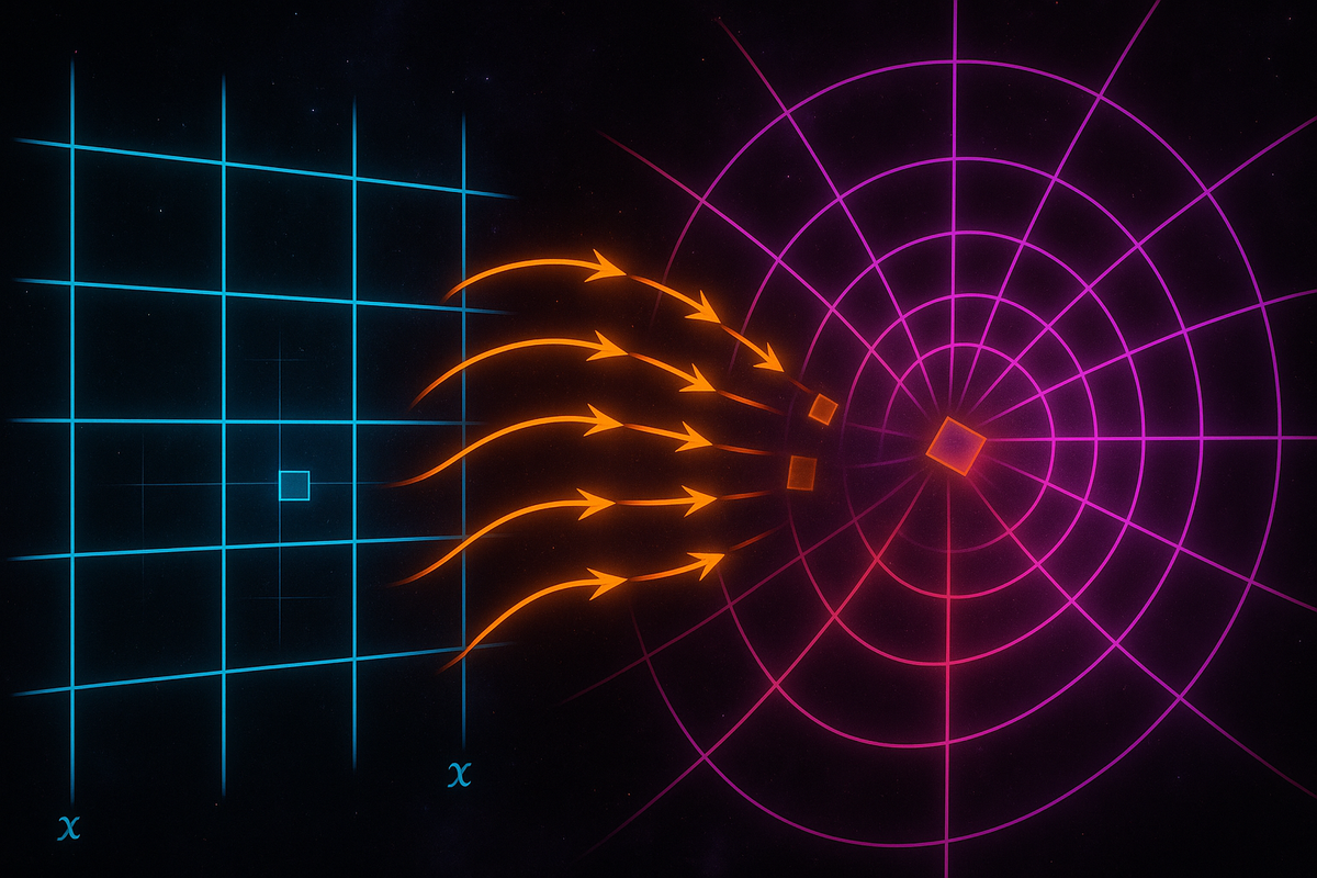
Different coordinate systems slice up space differently. Polar coordinates use concentric circles and radial lines; Cartesian uses a rectangular grid. The "shape" of infinitesimal regions changes.

The Jacobian determinant captures this: it's the factor by which area (or volume) elements expand or contract under the transformation.

This is why choosing coordinates to match the problem's symmetry is so powerful: the geometry becomes aligned with the coordinate grid, simplifying both the limits and the Jacobian.

What's Next

We've now covered the full integration toolkit:

• Double integrals over regions
• Triple integrals over volumes
• Jacobians for changing coordinates

Next, we turn to optimization: finding maxima and minima of functions subject to constraints.

This is where Lagrange multipliers come in—a technique that uses gradients to solve constrained optimization problems, foundational in economics, physics, engineering, and machine learning.

After that, we'll synthesize everything in a final article showing how the pieces of multivariable calculus fit together into a coherent framework for analyzing functions in multiple dimensions.

The Jacobian is the key that unlocks coordinate transformations, turning hard integrals into easy ones by choosing the right frame of reference.

With it mastered, you're equipped to integrate over any region, in any coordinate system.

Let's move to Lagrange multipliers.

Part 8 of the Multivariable Calculus series.

Previous: Triple Integrals: Integrating Through Volumes Next: Lagrange Multipliers: Optimization Under Constraints