Lagrange Multipliers: Optimization Under Constraints

You want to maximize a function f(x, y), but you can't choose x and y freely—they're constrained to satisfy g(x, y) = c.

This is constrained optimization: finding the best value of an objective function subject to a constraint.

Lagrange multipliers solve this by converting the constrained problem into an unconstrained one: instead of optimizing f subject to g = c, you optimize a new function—the Lagrangian—that encodes both the objective and the constraint.

This technique is foundational in economics (utility maximization under budget constraints), physics (equilibrium under constraints), machine learning (constrained loss minimization), and engineering (optimal design subject to physical limits).

The key insight: at a constrained extremum, the gradient of the objective function is parallel to the gradient of the constraint. Lagrange multipliers formalize this geometric condition into a solvable system of equations.

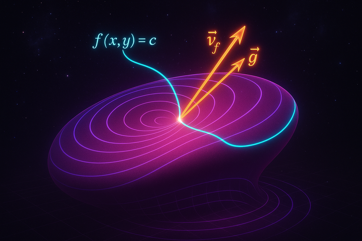
The Geometric Intuition: Gradients Must Align

Suppose you want to maximize f(x, y) subject to the constraint g(x, y) = c.

The constraint g(x, y) = c defines a curve in the xy-plane (a level curve of g).

You're restricted to moving along this curve. You want to find the point on the curve where f is largest.

Here's the key geometric insight: at the maximum, the level curve of f must be tangent to the constraint curve g(x, y) = c.

Why? If the level curves of f crossed the constraint curve, you could move along the constraint in the direction where f increases, so you wouldn't be at a maximum.

At the tangency point, both curves have the same tangent line, which means their normal vectors are parallel.

The gradient ∇f is perpendicular to level curves of f. The gradient ∇g is perpendicular to level curves of g.

If the curves are tangent, ∇f and ∇g must be parallel:

∇f = λ ∇g

for some scalar λ (called the Lagrange multiplier).

This is the core condition. Combined with the constraint g(x, y) = c, it gives you a system of equations to solve for x, y, and λ.

The Method: Setting Up the Lagrangian

To find extrema of f(x, y) subject to g(x, y) = c, follow these steps:

1. Form the Lagrangian: L(x, y, λ) = f(x, y) - λ(g(x, y) - c)
2. Compute partial derivatives and set them to zero:The first two equations enforce ∇f = λ ∇g. The third equation enforces the constraint g(x, y) = c.
   • ∂L/∂x = ∂f/∂x - λ ∂g/∂x = 0
   • ∂L/∂y = ∂f/∂y - λ ∂g/∂y = 0
   • ∂L/∂λ = -(g(x, y) - c) = 0
3. Solve the system for x, y, and λ.
4. Evaluate f at each solution to determine which is the maximum, which is the minimum.

The solutions (x, y) are the candidate points for constrained extrema.

Example 1: Maximize Area Given Perimeter

Maximize the area of a rectangle with perimeter 20.

Let x and y be the side lengths. The area is f(x, y) = xy.

The constraint is perimeter: g(x, y) = 2x + 2y = 20, or x + y = 10.

Lagrangian: L(x, y, λ) = xy - λ(x + y - 10)

Partial derivatives:

• ∂L/∂x = y - λ = 0 → y = λ
• ∂L/∂y = x - λ = 0 → x = λ
• ∂L/∂λ = -(x + y - 10) = 0 → x + y = 10

From the first two equations, x = y.

Substitute into the constraint: x + x = 10 → x = 5.

So y = 5 as well.

The maximum area occurs at x = y = 5, giving area = 25.

This makes geometric sense: among all rectangles with fixed perimeter, the square has the largest area.

Example 2: Minimize Distance to a Curve

Find the point on the line x + y = 4 closest to the origin.

Minimize f(x, y) = x² + y² (distance squared; minimizing this is equivalent to minimizing distance).

Constraint: g(x, y) = x + y = 4.

Lagrangian: L(x, y, λ) = x² + y² - λ(x + y - 4)

Partial derivatives:

• ∂L/∂x = 2x - λ = 0 → x = λ/2
• ∂L/∂y = 2y - λ = 0 → y = λ/2
• ∂L/∂λ = -(x + y - 4) = 0 → x + y = 4

From the first two equations, x = y.

Substitute into the constraint: x + x = 4 → x = 2, y = 2.

The closest point is (2, 2), with distance √(4 + 4) = 2√2.

Geometrically, the shortest path from the origin to the line is perpendicular to the line. The line x + y = 4 has slope -1, so the perpendicular has slope 1, passing through the origin: y = x. This intersects the line at (2, 2), confirming our answer.

Example 3: Maximize Utility Under Budget Constraint (Economics)

A consumer has utility u(x, y) = x^a y^b (Cobb-Douglas utility function), where x and y are quantities of two goods.

The budget constraint is p_x x + p_y y = I (total spending equals income I).

Maximize u subject to the budget constraint.

Lagrangian: L(x, y, λ) = x^a y^b - λ(p_x x + p_y y - I)

Partial derivatives:

• ∂L/∂x = a x^{a-1} y^b - λ p_x = 0
• ∂L/∂y = b x^a y^{b-1} - λ p_y = 0
• ∂L/∂λ = -(p_x x + p_y y - I) = 0

From the first equation: λ = (a x^{a-1} y^b) / p_x

From the second equation: λ = (b x^a y^{b-1}) / p_y

Equate:

(a x^{a-1} y^b) / p_x = (b x^a y^{b-1}) / p_y

Simplify:

a y / p_x = b x / p_y

Cross-multiply:

a p_y y = b p_x x

Solve for y:

y = (b p_x / a p_y) x

Substitute into the budget constraint:

p_x x + p_y [(b p_x / a p_y) x] = I

p_x x + (b p_x / a) x = I

p_x x [1 + b/a] = I

p_x x [(a + b)/a] = I

x = (a / (a + b)) (I / p_x)

Similarly:

y = (b / (a + b)) (I / p_y)

The consumer allocates a fraction a/(a+b) of income to good x and b/(a+b) to good y.

This is a classic result in microeconomics: Cobb-Douglas preferences lead to constant budget shares.

Lagrange multipliers turned a constrained optimization problem into a solvable algebraic system.

Multiple Constraints: Multiple Multipliers

If you have two constraints g(x, y, z) = c₁ and h(x, y, z) = c₂, the gradients ∇f, ∇g, and ∇h must all lie in the same plane (be linearly dependent):

∇f = λ ∇g + μ ∇h

You introduce one multiplier per constraint.

The Lagrangian becomes:

L(x, y, z, λ, μ) = f(x, y, z) - λ(g(x, y, z) - c₁) - μ(h(x, y, z) - c₂)

Setting ∂L/∂x, ∂L/∂y, ∂L/∂z, ∂L/∂λ, ∂L/∂μ all to zero gives a system of five equations in five unknowns.

Example: Minimize f(x, y, z) = x² + y² + z² subject to x + y + z = 1 and x - y + 2z = 2.

Lagrangian: L = x² + y² + z² - λ(x + y + z - 1) - μ(x - y + 2z - 2)

Partial derivatives:

• ∂L/∂x = 2x - λ - μ = 0
• ∂L/∂y = 2y - λ + μ = 0
• ∂L/∂z = 2z - λ - 2μ = 0
• ∂L/∂λ = -(x + y + z - 1) = 0
• ∂L/∂μ = -(x - y + 2z - 2) = 0

From the first three equations:

• 2x = λ + μ
• 2y = λ - μ
• 2z = λ + 2μ

Add the first two: 2x + 2y = 2λ → x + y = λ

Subtract: 2x - 2y = 2μ → x - y = μ

From the third: 2z = λ + 2μ = (x + y) + 2(x - y) = 3x - y

The constraints are:

• x + y + z = 1
• x - y + 2z = 2

Substitute 2z = 3x - y into the first constraint:

x + y + (3x - y)/2 = 1

2x + 2y + 3x - y = 2

5x + y = 2

Now use the second constraint:

x - y + 2z = 2

Substitute 2z = 3x - y:

x - y + (3x - y) = 2

4x - 2y = 2

2x - y = 1

So y = 2x - 1.

Substitute into 5x + y = 2:

5x + (2x - 1) = 2

7x = 3

x = 3/7

Then y = 2(3/7) - 1 = 6/7 - 7/7 = -1/7

And from 2z = 3x - y:

2z = 3(3/7) - (-1/7) = 9/7 + 1/7 = 10/7

z = 5/7

Check the constraints:

x + y + z = 3/7 - 1/7 + 5/7 = 7/7 = 1 ✓

x - y + 2z = 3/7 - (-1/7) + 10/7 = 3/7 + 1/7 + 10/7 = 14/7 = 2 ✓

The minimum value is f(3/7, -1/7, 5/7) = (3/7)² + (-1/7)² + (5/7)² = (9 + 1 + 25)/49 = 35/49 = 5/7.

Multiple constraints just mean more equations, solved systematically.

Interpretation of λ: Sensitivity to the Constraint

The Lagrange multiplier λ has an economic interpretation: it's the rate of change of the optimal value with respect to the constraint.

If you relax the constraint slightly (change c to c + Δc), the optimal value of f changes by approximately λ Δc.

In economics, λ is the "shadow price" or "marginal utility of wealth"—how much additional utility you'd gain from one more unit of budget.

In optimization, λ tells you how sensitive the solution is to the constraint: if λ is large, tightening the constraint hurts a lot; if λ is small, the constraint is nearly slack.

Inequality Constraints: KKT Conditions

Lagrange multipliers handle equality constraints (g = c). What about inequality constraints (g ≤ c)?

This requires the Karush-Kuhn-Tucker (KKT) conditions, which generalize Lagrange multipliers.

The key idea: if the constraint is not active (g < c), it doesn't affect the optimum, and you can ignore it. If the constraint is active (g = c), it acts like an equality constraint, and you use a Lagrange multiplier.

The KKT conditions include:

• Stationarity: ∇f = Σ λᵢ ∇gᵢ (as before)
• Primal feasibility: gᵢ(x) ≤ cᵢ (constraints are satisfied)
• Dual feasibility: λᵢ ≥ 0 (multipliers are non-negative)
• Complementary slackness: λᵢ (gᵢ(x) - cᵢ) = 0 (if constraint is inactive, λᵢ = 0; if λᵢ > 0, constraint is active)

This framework is central to convex optimization, linear programming, and machine learning.

For this article, we focus on equality constraints, but KKT conditions are the natural extension.

When Lagrange Multipliers Fail

Lagrange multipliers find critical points, not necessarily maxima or minima.

You must check:

1. Are there multiple critical points? Evaluate f at each to determine which is max/min.
2. Are there boundary effects? If the constraint region has boundaries, check them separately.
3. Is the problem well-posed? If the constraint is incompatible with the domain, there might be no solution.

Also, Lagrange multipliers assume the constraints are smooth (differentiable) and that ∇g ≠ 0 (the constraint is "regular").

If ∇g = 0 at a point, that point is a singularity of the constraint, and the method may not apply.

Example 4: Maximize Volume of a Box with Fixed Surface Area

Maximize the volume V = xyz of a rectangular box subject to fixed surface area S = 2(xy + xz + yz).

Constraint: g(x, y, z) = xy + xz + yz = S/2.

Objective: f(x, y, z) = xyz.

Lagrangian: L = xyz - λ(xy + xz + yz - S/2)

Partial derivatives:

• ∂L/∂x = yz - λ(y + z) = 0 → yz = λ(y + z)
• ∂L/∂y = xz - λ(x + z) = 0 → xz = λ(x + z)
• ∂L/∂z = xy - λ(x + y) = 0 → xy = λ(x + y)
• ∂L/∂λ = -(xy + xz + yz - S/2) = 0

From the first equation: yz/(y + z) = λ

From the second equation: xz/(x + z) = λ

Equate:

yz/(y + z) = xz/(x + z)

If z ≠ 0, divide by z:

y/(y + z) = x/(x + z)

Cross-multiply:

y(x + z) = x(y + z)

yx + yz = xy + xz

yz = xz

If z ≠ 0, then y = x.

Similarly, comparing the second and third equations gives x = z.

So x = y = z.

Substitute into the constraint:

x² + x² + x² = S/2

3x² = S/2

x² = S/6

x = √(S/6)

The box is a cube with side length √(S/6).

Volume = x³ = (S/6)^(3/2).

This is the maximum volume: among all boxes with fixed surface area, the cube has the largest volume.

Lagrange Multipliers in Higher Dimensions

The method generalizes to any number of variables and constraints.

Minimize/maximize f(x₁, x₂, ..., xₙ) subject to gᵢ(x₁, ..., xₙ) = cᵢ for i = 1, ..., m (with m < n).

Lagrangian: L = f - Σ λᵢ (gᵢ - cᵢ)

Set ∂L/∂x_j = 0 for all j and ∂L/∂λᵢ = 0 for all i.

You get n + m equations in n + m unknowns (the xⱼ's and λᵢ's).

This is the standard approach in high-dimensional optimization.

Connection to Gradient Descent with Constraints

In unconstrained optimization, you follow the gradient ∇f to find extrema.

In constrained optimization, you can't move freely—you're restricted to the constraint surface.

Lagrange multipliers find where the projected gradient onto the constraint surface is zero—where you can't increase f by moving along the constraint.

In machine learning, when you optimize with constraints (e.g., weights must sum to 1), you often use projected gradient descent: take a gradient step, then project back onto the constraint.

Lagrange multipliers give the exact condition for the constrained optimum, which gradient methods approximate iteratively.

The Conceptual Core: Turning Constraints Into Dimensions

The Lagrange multiplier λ converts the constraint from a restriction into an additional dimension in the problem.

Instead of optimizing f subject to g = c (a constrained problem in x, y), you optimize L (an unconstrained problem in x, y, λ).

The constraint reemerges as a stationarity condition: ∂L/∂λ = 0 enforces g = c.

This is a powerful trick: constraints are just additional variables whose stationarity conditions encode the constraints.

This perspective unifies constrained and unconstrained optimization, and extends to duality theory in convex optimization.

Practical Workflow

When faced with a constrained optimization problem:

1. Identify the objective f (what you want to maximize/minimize).
2. Identify the constraints g (what equations must hold).
3. Write the Lagrangian L = f - Σ λᵢ (gᵢ - cᵢ).
4. Compute all partial derivatives ∂L/∂x, ∂L/∂y, ..., ∂L/∂λᵢ.
5. Set them all to zero to get a system of equations.
6. Solve the system (algebraically, numerically, or symbolically).
7. Evaluate f at the solutions to determine which is max/min.
8. Check boundary cases or constraints if the problem has them.

This is systematic and scales to arbitrarily complex problems.

What's Next

Lagrange multipliers complete the optimization toolkit for multivariable calculus:

• Unconstrained optimization: set ∇f = 0
• Constrained optimization: set ∇f = λ ∇g

We've now covered differentiation (partial derivatives, gradients, directional derivatives, chain rule), integration (double, triple, Jacobians), and optimization (critical points, Lagrange multipliers).

Next, we synthesize: how do all these pieces fit together? What's the overarching structure of multivariable calculus?

The final article will pull the threads together, showing how multivariable calculus is a unified framework for analyzing functions in higher dimensions—how to differentiate them, integrate them, optimize them, and transform them.

Lagrange multipliers are the crown jewel of constrained optimization. With them, you can solve problems where the gradient alone isn't enough—where the constraints shape the solution.

Let's synthesize.

Part 9 of the Multivariable Calculus series.

Previous: Change of Variables: Jacobians and Coordinate Transforms Next: Synthesis: Multivariable Calculus as the Language of Fields