The Law of Large Numbers: Why Averages Stabilize

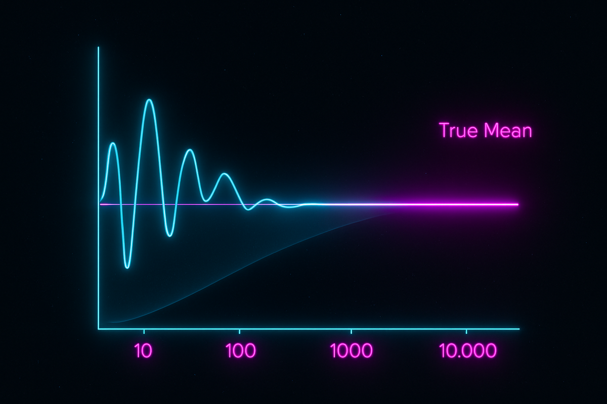
Flip a fair coin 10 times. You might get 7 heads, or 4, or 6. Lots of variation.

Flip it 10,000 times. You'll get very close to 50% heads. The variation shrinks.

This isn't just observation—it's mathematical law. The Law of Large Numbers guarantees that sample averages converge to expected values as sample sizes grow.

This theorem is why statistics works.

The Statement

Let X₁, X₂, X₃, ... be independent random variables with the same distribution, with mean μ.

Define the sample average: X̄ₙ = (X₁ + X₂ + ... + Xₙ) / n

Law of Large Numbers: X̄ₙ → μ as n → ∞

The sample average converges to the true mean. The more samples you have, the closer your average gets to the expected value.

Two Versions

Weak Law of Large Numbers:

For any ε > 0: P(|X̄ₙ - μ| > ε) → 0 as n → ∞

"Convergence in probability." The probability of being far from μ vanishes.

Strong Law of Large Numbers:

P(X̄ₙ → μ) = 1

"Almost sure convergence." The sample average converges to μ with probability 1.

The strong version is stronger (obviously). It says not just that large deviations become unlikely, but that convergence actually happens.

Why It Works: Intuition

Each Xᵢ varies around μ. Some are above, some below.

When you average many of them, the "aboves" and "belows" tend to cancel. The more you average, the more cancellation.

The variance of the average is Var(X̄ₙ) = σ²/n. As n grows, variance shrinks to zero. The average becomes increasingly concentrated around μ.

Why It Works: Proof Sketch

Chebyshev's inequality:

P(|X̄ₙ - μ| ≥ ε) ≤ Var(X̄ₙ) / ε² = σ² / (nε²)

As n → ∞, this bound → 0.

So P(|X̄ₙ - μ| ≥ ε) → 0 for any ε > 0.

This proves the weak law. The strong law requires more machinery (Borel-Cantelli lemma).

Examples

Coin Flips:

Let Xᵢ = 1 if heads, 0 if tails. E[Xᵢ] = 0.5.

X̄ₙ = (number of heads) / n → 0.5 as n → ∞.

Die Rolls:

E[single roll] = 3.5.

Average of n rolls → 3.5 as n → ∞.

Stock Returns:

Daily returns vary wildly. But the average return over many days converges to the expected daily return.

What LLN Doesn't Say

Not about single outcomes: The law says nothing about any individual trial. The next coin flip is still 50-50.

Not about short runs: With 10 flips, substantial deviation from 50% is common. LLN is about the limit as n → ∞.

Not recovery from bad starts: If you're down in gambling, LLN doesn't mean you'll "even out." Future games have zero expected gain; you don't recover past losses.

The Gambler's Fallacy—thinking that after many heads, tails is "due"—misunderstands LLN. Each flip is independent. The convergence happens by dilution (many future trials swamp past anomalies), not correction.

Requirements

Finite mean: If E[|X|] = ∞, LLN fails. The Cauchy distribution has no mean, and averages of Cauchy samples don't converge.

Independence (or weak dependence): Highly dependent samples can violate LLN. If all samples are identical, X̄ₙ = X₁ forever.

Identical distribution: Needed in the basic form. There are generalizations for non-identical distributions.

Applications

Sampling: LLN justifies using sample means to estimate population means. With enough data, the sample mean approximates the true mean.

Simulation: Monte Carlo methods estimate integrals by averaging random samples. LLN guarantees convergence.

Insurance: Individual claims are unpredictable. Average claims converge to expected claims. Insurers price based on expected values and profit reliably.

Quality Control: Average defect rates converge to true defect rates. Large enough samples accurately estimate quality.

Casinos: Individual gamblers win or lose unpredictably. But the casino's average take converges to the house edge. Casinos make predictable money.

The Rate of Convergence

LLN guarantees convergence but doesn't say how fast.

Standard error: σ/√n

The sample mean has standard deviation σ/√n. To halve your uncertainty, you need 4× as many samples.

Chebyshev's bound: P(|X̄ₙ - μ| ≥ ε) ≤ σ²/(nε²)

This gives explicit (if loose) bounds on deviation probability.

Central Limit Theorem: (X̄ₙ - μ) × √n → Normal(0, σ²)

Not only does X̄ₙ converge to μ, but the distribution of fluctuations around μ is normal. The CLT gives more precise probability statements than Chebyshev.

Extensions

Weak dependence: LLN holds if samples are weakly dependent (correlations decay fast enough with distance).

Different distributions: If Xᵢ have different means μᵢ, the average converges to the average of means (under technical conditions).

Empirical distributions: The proportion of samples falling in any set converges to the true probability of that set. This is the Glivenko-Cantelli theorem—the empirical distribution converges to the true distribution.

Philosophical Implications

Frequentist interpretation: LLN is why "probability = long-run frequency" makes sense. Run the experiment many times; the frequency of an event converges to its probability.

Justification for statistics: LLN provides theoretical backing for using samples to learn about populations. It's not just a good idea—it's mathematically guaranteed to work (given enough samples).

Order from randomness: Individual events are unpredictable, yet aggregates are predictable. The chaos at the micro level produces regularity at the macro level.

The Limit and Beyond

LLN tells us about the limit. The Central Limit Theorem tells us about the approach to the limit—the distribution of deviations before convergence.

Together, they're the theoretical foundation of frequentist statistics. Sample averages converge (LLN), and their fluctuations are approximately normal (CLT).

This is Part 10 of the Probability series. Next: "The Central Limit Theorem: Why Everything Is Normal."

Part 10 of the Probability series.

Previous: Common Distributions: Binomial Poisson and Beyond Next: The Central Limit Theorem: Why the Bell Curve Rules