Linear First-Order: The Integrating Factor Method

Linear first-order differential equations are everywhere. Electric circuits, mixing problems, population models with immigration, Newton's cooling with external heat sources—all linear first-order.

Standard form: dy/dx + P(x)y = Q(x)

The key word is "linear." The unknown function y and its derivative dy/dx appear to the first power only. No y², no (dy/dx)², no products like y·(dy/dx).

This linearity unlocks a systematic solution method: the integrating factor technique.

What Makes an Equation Linear

A first-order ODE is linear if it can be written as:

dy/dx + P(x)y = Q(x)

where P(x) and Q(x) are functions of x alone (or constants).

Linear examples:

dy/dx + 2y = 3 (P(x) = 2, Q(x) = 3)

dy/dx + (1/x)y = x² (P(x) = 1/x, Q(x) = x²)

dy/dx + (cos x)y = sin x (P(x) = cos x, Q(x) = sin x)

Nonlinear examples:

dy/dx + y² = x (y² makes it nonlinear)

dy/dx + xy = y(dy/dx) (product of y and dy/dx)

Linearity is structural. If y and dy/dx appear only to the first power and not multiplied together, it's linear.

Standard Form

Always convert to standard form: dy/dx + P(x)y = Q(x)

Example: x dy/dx - 2y = x³

Divide by x: dy/dx - (2/x)y = x²

Now it's in standard form with P(x) = -2/x and Q(x) = x².

Standard form makes the solution method mechanical.

The Integrating Factor Method

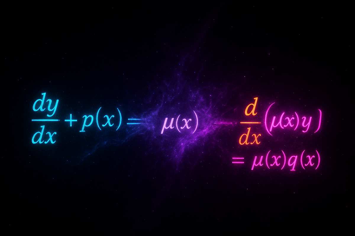
The idea: multiply the equation by a cleverly chosen function μ(x) that makes the left side a perfect derivative.

If dy/dx + P(x)y = Q(x), multiply by μ(x):

μ(dy/dx) + μP(x)y = μQ(x)

We want the left side to equal d/dx[μy].

By product rule: d/dx[μy] = μ(dy/dx) + (dμ/dx)y

Comparing with our equation, we need:

μP(x)y = (dμ/dx)y

So: dμ/dx = μP(x)

This is a separable equation in μ:

dμ/μ = P(x)dx

ln|μ| = ∫P(x)dx

μ(x) = e^(∫P(x)dx)

This is the integrating factor.

The Solution Process

Step 1: Write in standard form dy/dx + P(x)y = Q(x).

Step 2: Compute integrating factor μ(x) = e^(∫P(x)dx).

Step 3: Multiply equation by μ:

μ(dy/dx) + μP(x)y = μQ(x)

Left side simplifies to d/dx[μy], so:

d/dx[μy] = μQ(x)

Step 4: Integrate both sides:

μy = ∫μQ(x)dx + C

Step 5: Solve for y:

y = (1/μ)[∫μQ(x)dx + C]

Done.

Example 1: Basic Linear Equation

Solve: dy/dx + 2y = 6

Step 1: Already in standard form. P(x) = 2, Q(x) = 6.

Step 2: Integrating factor:

μ = e^(∫2 dx) = e^(2x)

Step 3: Multiply by μ:

e^(2x)(dy/dx) + 2e^(2x)y = 6e^(2x)

Left side is d/dx[e^(2x)y]:

d/dx[e^(2x)y] = 6e^(2x)

Step 4: Integrate:

e^(2x)y = ∫6e^(2x)dx = 3e^(2x) + C

Step 5: Solve for y:

y = 3 + Ce^(-2x)

General solution: y = 3 + Ce^(-2x)

As x → ∞, y → 3 (equilibrium value).

Example 2: Variable Coefficients

Solve: dy/dx + (1/x)y = 3x

Step 1: Standard form. P(x) = 1/x, Q(x) = 3x.

Step 2: Integrating factor:

μ = e^(∫(1/x)dx) = e^(ln|x|) = |x| = x (assuming x > 0)

Step 3: Multiply by μ = x:

x(dy/dx) + y = 3x²

Left side is d/dx[xy]:

d/dx[xy] = 3x²

Step 4: Integrate:

xy = ∫3x²dx = x³ + C

Step 5: Solve for y:

y = x² + C/x

General solution: y = x² + C/x

Example 3: Initial Value Problem

Solve: dy/dx - y = e^x with y(0) = 2

Step 1: Standard form. P(x) = -1, Q(x) = e^x.

Step 2: Integrating factor:

μ = e^(∫-1 dx) = e^(-x)

Step 3: Multiply by e^(-x):

e^(-x)(dy/dx) - e^(-x)y = e^(-x)·e^x = 1

Left side is d/dx[e^(-x)y]:

d/dx[e^(-x)y] = 1

Step 4: Integrate:

e^(-x)y = x + C

Step 5: Solve for y:

y = xe^x + Ce^x

Step 6: Apply initial condition y(0) = 2:

2 = 0 + C, so C = 2.

Particular solution: y = xe^x + 2e^x = e^x(x + 2)

Why It Works

The integrating factor μ(x) converts the left side into a derivative:

μ(dy/dx) + μP(x)y = d/dx[μy]

This is possible because:

d/dx[μy] = μ(dy/dx) + (dμ/dx)y

If we choose μ such that dμ/dx = μP(x), then:

d/dx[μy] = μ(dy/dx) + μP(x)y

which matches our equation after multiplying by μ.

It's a designed construction. We engineer μ specifically to collapse the left side into a single derivative, which we can then integrate directly.

Homogeneous vs Nonhomogeneous

A linear equation is homogeneous if Q(x) = 0:

dy/dx + P(x)y = 0

Homogeneous equations are separable:

dy/y = -P(x)dx

ln|y| = -∫P(x)dx + C₁

y = Ce^(-∫P(x)dx)

This is the complementary solution (also called homogeneous solution).

A linear equation is nonhomogeneous if Q(x) ≠ 0:

dy/dx + P(x)y = Q(x)

The general solution is:

y = y_c + y_p

where:

• y_c = complementary solution (solution to homogeneous equation)
• y_p = particular solution (any solution to nonhomogeneous equation)

The integrating factor method automatically gives you the full general solution.

Example: Homogeneous Equation

Solve: dy/dx + 3y = 0

This is separable:

dy/y = -3dx

ln|y| = -3x + C₁

y = Ce^(-3x)

Alternatively, using integrating factor:

μ = e^(∫3 dx) = e^(3x)

Multiply: e^(3x)(dy/dx) + 3e^(3x)y = 0

d/dx[e^(3x)y] = 0

Integrate: e^(3x)y = C

y = Ce^(-3x)

Same answer, two methods.

Applications

RC Circuit:

Voltage across capacitor: dV/dt + V/(RC) = V_in/R

This is linear first-order. Using integrating factor with P = 1/(RC), you solve for V(t).

Mixing with Inflow/Outflow:

Tank with inflow concentration c_in and outflow concentration Q/V:

dQ/dt + (r/V)Q = r·c_in

Linear first-order in Q.

Newton's Cooling with External Heat:

dT/dt + kT = kT_a + H(t)

where H(t) is external heating. Linear in T.

All solved by integrating factor.

When Integrating Factor Gets Messy

Sometimes ∫μQ(x)dx can't be computed in elementary functions.

Example: dy/dx + y = e^(x²)

Integrating factor: μ = e^x

Multiply: d/dx[e^x y] = e^x · e^(x²) = e^(x² + x)

Integrate: e^x y = ∫e^(x² + x)dx

But ∫e^(x² + x)dx has no elementary antiderivative.

In such cases:

• Leave answer in integral form: y = e^(-x)∫e^(x² + x)dx
• Use numerical integration
• Use series methods

The method still works conceptually; it's just the integration that's hard.

Variation of Parameters

Another perspective: variation of parameters.

For homogeneous equation dy/dx + P(x)y = 0, solution is y = Ce^(-∫P dx).

For nonhomogeneous, let the "constant" vary: y = C(x)e^(-∫P dx).

Substitute into original equation and solve for C(x). This gives the same result as integrating factor but with different framing.

It's conceptually elegant: the nonhomogeneous term perturbs the constant into a function.

Reduction of Order Connection

The integrating factor method is a special case of a more general technique called reduction of order, which works for higher-order linear equations.

For first-order, it's overkill. But the underlying principle—multiplying by a function to simplify structure—extends to second-order and beyond.

Standard Mistakes

Mistake 1: Forgetting to convert to standard form before computing μ.

If equation is 2dy/dx + 4y = 6, you must divide by 2 first: dy/dx + 2y = 3.

Mistake 2: Dropping the constant of integration.

When you integrate d/dx[μy] = μQ, you get μy = ∫μQ dx + C. Don't forget +C.

Mistake 3: Not simplifying μ.

If ∫P dx = ln|x|, then μ = e^(ln|x|) = |x|. Often you can drop absolute value by choosing domain (e.g., x > 0).

Mistake 4: Misidentifying P(x) and Q(x).

In dy/dx + P(x)y = Q(x), everything multiplying y goes into P, everything else into Q.

When to Use Integrating Factor

Use integrating factor if:

• Equation is first-order
• Equation is linear (y and dy/dx to first power only)
• You can integrate ∫P(x)dx and ∫μQ(x)dx

If equation is nonlinear, integrating factor won't work. You'd need other techniques (Bernoulli substitution, exact equations, numerical methods).

Summary of Method

1. Write dy/dx + P(x)y = Q(x)
2. Compute μ(x) = e^(∫P(x)dx)
3. Multiply equation by μ
4. Recognize left side as d/dx[μy]
5. Integrate: μy = ∫μQ dx + C
6. Solve for y

It's algorithmic. Once you identify it as linear, the method is mechanical.

Next up: second-order linear ODEs, where things get more complex but the principles extend.

Part 5 of the Differential Equations series.

Previous: Separable Equations: When Variables Can Be Pulled Apart Next: Second-Order Linear: Springs and Oscillations