Maxwell's Equations: Vector Calculus in Electromagnetism

Maxwell's equations are vector calculus distilled to four lines. They completely describe classical electromagnetism—how electric and magnetic fields are created, how they interact, and how they propagate as light.

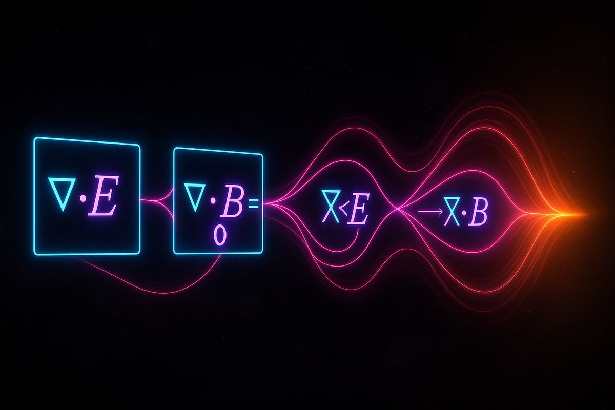
Here they are in differential form:

∇ · E = ρ/ε₀ (Gauss's law) ∇ · B = 0 (no magnetic monopoles) ∇ × E = -∂B/∂t (Faraday's law) ∇ × B = μ₀J + μ₀ε₀∂E/∂t (Ampère-Maxwell law)

Two divergence equations, two curl equations. Four del operations. That's it.

Before Maxwell, electricity and magnetism were separate phenomena described by verbose verbal laws. Maxwell unified them, reformulated them in vector calculus, and discovered that light is an electromagnetic wave. This is one of the greatest achievements in physics—and it only makes sense with vector calculus.

The Four Equations

Gauss's Law: ∇ · E = ρ/ε₀

The divergence of the electric field equals the charge density (up to a constant ε₀, the permittivity of free space).

Electric charges create electric field. Positive charges are sources (∇ · E > 0). Negative charges are sinks (∇ · E < 0). No charges means zero divergence.

This is a local differential statement. The integral form (from the Divergence Theorem) is:

∫∫S E · dS = Q{enclosed} / ε₀

Flux through a closed surface equals enclosed charge. That's the experimentally observed Gauss's Law. The differential form is the fundamental equation.

No Magnetic Monopoles: ∇ · B = 0

The divergence of the magnetic field is zero everywhere.

Magnetic field has no sources or sinks. There are no magnetic charges (as far as we know). Magnetic field lines always form closed loops—they never begin or end.

This is why magnets always have north and south poles. Cut a magnet in half, and you get two smaller magnets, each with north and south. You can't isolate a magnetic monopole.

The integral form:

∫∫_S B · dS = 0

Flux through any closed surface is zero. What goes in comes out.

Faraday's Law: ∇ × E = -∂B/∂t

The curl of the electric field equals the negative rate of change of the magnetic field.

A changing magnetic field creates a curling electric field. This is electromagnetic induction—the principle behind generators, transformers, and inductors.

The minus sign is Lenz's law: the induced electric field opposes the change in magnetic field.

The integral form (from Stokes' Theorem):

∫_C E · dr = -d/dt ∫∫_S B · dS

The circulation of electric field around a loop equals the negative rate of change of magnetic flux through the loop. This is the experimentally observed law. The differential form is the fundamental equation.

Ampère-Maxwell Law: ∇ × B = μ₀J + μ₀ε₀∂E/∂t

The curl of the magnetic field is driven by current density J and the rate of change of the electric field.

The first term (μ₀J) is Ampère's original law: electric current creates curling magnetic field. This is how electromagnets work.

The second term (μ₀ε₀∂E/∂t) is Maxwell's addition: a changing electric field creates curling magnetic field, just like current does. This is the displacement current.

Maxwell's addition was crucial. Without it, the equations are inconsistent (they violate charge conservation). With it, they predict electromagnetic waves traveling at speed c = 1/√(μ₀ε₀)—which turns out to be the speed of light. Maxwell realized light is an electromagnetic wave.

The integral form (from Stokes' Theorem):

∫C B · dr = μ₀I{enclosed} + μ₀ε₀ d/dt ∫∫_S E · dS

Circulation of magnetic field around a loop equals the current through the loop plus the rate of change of electric flux. This generalizes Ampère's law to include displacement current.

The Structure

Notice the pattern:

• Two divergence equations: ∇ · E and ∇ · B. These describe sources.
• Two curl equations: ∇ × E and ∇ × B. These describe rotation and dynamics.

Divergence tells you where fields come from. Curl tells you how fields swirl and interact.

Electric field has sources (charges). Magnetic field doesn't. Both have curl, driven by time-varying fields and currents.

The equations are coupled. E creates ∇ × B (via ∂E/∂t). B creates ∇ × E (via ∂B/∂t). They're intertwined. A changing electric field creates a magnetic field, which creates an electric field, which creates a magnetic field—this feedback loop is an electromagnetic wave.

Electromagnetic Waves

In vacuum (ρ = 0, J = 0), Maxwell's equations simplify:

∇ · E = 0 ∇ · B = 0 ∇ × E = -∂B/∂t ∇ × B = μ₀ε₀∂E/∂t

Take the curl of Faraday's law:

∇ × (∇ × E) = -∂/∂t (∇ × B)

Use the vector identity ∇ × (∇ × E) = ∇(∇ · E) - ∇²E. Since ∇ · E = 0:

-∇²E = -∂/∂t (μ₀ε₀ ∂E/∂t) = -μ₀ε₀ ∂²E/∂t²

So:

∇²E = μ₀ε₀ ∂²E/∂t²

This is the wave equation. Electric field propagates as a wave with speed 1/√(μ₀ε₀) = c.

Similarly, taking the curl of Ampère-Maxwell law gives:

∇²B = μ₀ε₀ ∂²B/∂t²

Magnetic field also propagates as a wave at speed c.

Electromagnetic waves are oscillations of E and B fields traveling through space. Light, radio waves, X-rays—all electromagnetic waves, all solutions to Maxwell's equations.

The Constants

ε₀ (permittivity of free space): ~8.85 × 10⁻¹² F/m. Relates electric field to charge density.

μ₀ (permeability of free space): 4π × 10⁻⁷ H/m. Relates magnetic field to current density.

c (speed of light): c = 1/√(μ₀ε₀) ≈ 3 × 10⁸ m/s.

These constants link the equations to physical units. They're fundamental constants of nature.

Charge Conservation

Take the divergence of Ampère-Maxwell law:

∇ · (∇ × B) = ∇ · (μ₀J + μ₀ε₀∂E/∂t)

The left side is zero (divergence of curl is always zero). So:

0 = μ₀ ∇ · J + μ₀ε₀ ∂/∂t (∇ · E)

Using Gauss's law ∇ · E = ρ/ε₀:

0 = ∇ · J + ∂ρ/∂t

This is the continuity equation: ∂ρ/∂t + ∇ · J = 0.

Charge is conserved. The rate of change of charge density equals the negative divergence of current. Charge can't be created or destroyed—it just flows.

Maxwell's equations automatically enforce charge conservation. This is why the displacement current term was necessary. Without it, the equations would violate charge conservation.

Gauge Freedom and Potentials

Electric and magnetic fields can be expressed in terms of potentials:

E = -∇V - ∂A/∂t B = ∇ × A

where V is the scalar potential (voltage) and A is the vector potential.

Why? Because ∇ · B = 0 implies B is a curl (divergence of curl is zero). And ∇ × E = -∂B/∂t implies E + ∂A/∂t is curl-free, so it's a gradient.

The potentials V and A aren't unique. You can add a gradient to A and adjust V accordingly without changing E or B. This is gauge freedom—a fundamental feature of electromagnetism that becomes central in quantum mechanics and gauge theories.

Maxwell's equations in terms of potentials are more complicated but reveal deeper structure. In quantum mechanics, the potentials are the primary objects; the fields are derived.

Energy and Momentum

Electromagnetic fields carry energy and momentum.

Energy density: u = (1/2)(ε₀E² + B²/μ₀)

Energy flux (Poynting vector): S = (1/μ₀) E × B

Momentum density: g = ε₀(E × B) = S/c²

These quantities satisfy conservation laws derived from Maxwell's equations. The Poynting vector points in the direction of energy flow—for a plane wave, it's the direction of propagation.

Light exerts pressure. Electromagnetic waves carry momentum. This is why solar sails work—light from the sun pushes on the sail.

Why Vector Calculus is Essential

Without vector calculus, Maxwell's equations are a mess. In component form, the four vector equations expand to 12 scalar equations with dozens of partial derivatives.

∂E_x/∂x + ∂E_y/∂y + ∂E_z/∂z = ρ/ε₀ ∂B_x/∂x + ∂B_y/∂y + ∂B_z/∂z = 0 ∂E_z/∂y - ∂E_y/∂z = -∂B_x/∂t ... (nine more equations)

Completely opaque. You can't see the structure. You can't see the symmetry. You can't see that light is an electromagnetic wave.

Vector calculus compresses this into:

∇ · E = ρ/ε₀ ∇ · B = 0 ∇ × E = -∂B/∂t ∇ × B = μ₀J + μ₀ε₀∂E/∂t

Now the structure is visible. Two divergence equations, two curl equations. Sources and rotation. Coupling via time derivatives. Symmetry between E and B (almost—there are no magnetic charges, but otherwise symmetric).

The vector calculus formulation isn't just notation. It reveals the conceptual unity.

The Physical Meaning

∇ · E = ρ/ε₀: Charges create diverging electric field. Where there's charge, field lines radiate out (or converge in).

∇ · B = 0: Magnetic field has no sources. Field lines loop back on themselves.

∇ × E = -∂B/∂t: Changing magnetic field creates swirling electric field. This is induction.

∇ × B = μ₀J + μ₀ε₀∂E/∂t: Current and changing electric field create swirling magnetic field. This is how electromagnets and waves work.

Each equation has a clear geometric meaning. Divergence is spreading. Curl is swirling. Time derivatives are change. The equations describe how fields spread, swirl, and evolve.

Historical Impact

Before Maxwell, there were separate laws for electricity and magnetism: Coulomb's law, Ampère's law, Faraday's law of induction, etc. These were empirical observations, disconnected.

Maxwell unified them. He introduced the displacement current (the ∂E/∂t term), making the equations consistent. He reformulated everything in vector calculus. And he discovered that light is an electromagnetic wave—a prediction confirmed by Hertz's experiments.

This was a paradigm shift. Electricity, magnetism, and optics were unified. The speed of light emerged from electric and magnetic constants. And vector calculus became the language of field theory.

Later, Einstein's special relativity revealed that E and B are components of a single electromagnetic field tensor. Maxwell's equations are Lorentz-invariant—they're the same in all inertial frames. This deep symmetry was hidden in the original formulation but visible in the vector calculus version.

Applications

Maxwell's equations describe every electromagnetic phenomenon:

• Static fields (electrostatics, magnetostatics)
• Circuits (voltage, current, inductance, capacitance)
• Electromagnetic waves (light, radio, X-rays)
• Antennas and radiation
• Waveguides and transmission lines
• Plasma physics and magnetohydrodynamics
• Optics (reflection, refraction, diffraction)

Every device that uses electricity—phones, computers, power grids, MRI machines, radio transmitters—operates according to Maxwell's equations.

The equations are also the foundation for quantum electrodynamics (QED), the quantum field theory of light and electrons. In QED, the fields are quantized, but the classical equations remain the starting point.

The Beauty

Maxwell's equations are considered one of the most beautiful results in physics. Four lines that unify electricity, magnetism, and light. Written in vector calculus, they reveal deep symmetry and conceptual clarity.

They're also a testament to the power of mathematics. Maxwell didn't discover new experimental facts—he reformulated known laws in a consistent framework. The displacement current was a mathematical necessity (to preserve charge conservation), not an experimental observation. Yet it turned out to be real, and it predicted electromagnetic waves.

This is mathematics guiding physics. The structure of the equations revealed new phenomena. Vector calculus wasn't just notation—it was a tool for thought.

Why This Matters for Learning Vector Calculus

Maxwell's equations are the payoff. They're where all the tools of vector calculus—gradient, divergence, curl, del, line integrals, surface integrals, Green's Theorem, Stokes' Theorem, the Divergence Theorem—come together in a single coherent theory.

Understanding Maxwell's equations requires understanding every piece of vector calculus. The divergence equations use Gauss's Law via the Divergence Theorem. The curl equations use Faraday's Law and Ampère's Law via Stokes' Theorem. The fields themselves are gradients and curls of potentials.

If you can read Maxwell's equations and understand what each symbol means geometrically, you've mastered vector calculus. You're not just manipulating formulas—you're reading the language of field theory.

And that's the ultimate goal: not just to compute integrals, but to understand how fields behave, how they spread and swirl, how they create and propagate waves. Maxwell's equations are the synthesis. Everything else in this series is preparation for understanding them.

Once you see electromagnetism as four del operations, you see the unity. And you see why vector calculus exists in the first place.

Part 11 of the Vector Calculus series.

Previous: The Divergence Theorem: From Surface Flux to Volume Sources Next: Synthesis: Vector Calculus as the Language of Physics