Message Passing and Belief Propagation in Active Inference

Series: Active Inference Applied | Part: 4 of 10

Building a generative model is one thing. Computing with it efficiently is another. Active inference agents need to infer hidden states, evaluate policies, and update beliefs in real time—all while minimizing something called variational free energy. The mathematics behind this is elegant but computationally intractable in its raw form. You can't just write down Bayes' rule and expect a robot to plan its actions at 30 Hz.

This is where message passing enters the picture. It's the computational architecture that makes active inference tractable—the bridge between theoretical elegance and working code. By representing probabilistic models as factor graphs and propagating beliefs through local computations, message passing algorithms turn inference from an exponential nightmare into something you can actually run on hardware.

If active inference is the theory of how systems minimize surprise, message passing is the algorithm that makes it computable. And the specific variant that powers most modern implementations—belief propagation—has a remarkable property: it finds approximate solutions to otherwise impossible problems by having nodes in a graph talk to their neighbors.

The Inference Problem: Why Brute Force Doesn't Scale

Active inference agents must perform probabilistic inference: given observations and a generative model, what are the most likely hidden states of the world? This sounds straightforward until you realize the computational requirements.

Exact Bayesian inference requires marginalizing over all possible combinations of hidden variables. For a model with just 10 binary variables, that's 1,024 states to consider. For 20 variables, it's over a million. For 30, it's over a billion. Real-world models routinely have hundreds or thousands of variables across multiple time steps. Exact inference becomes computationally intractable—the number of calculations grows exponentially with model complexity.

This is the curse of dimensionality, and it's why you can't just implement Bayes' rule directly. The brain has roughly 86 billion neurons, each with thousands of connections. If inference required considering all possible states of this system, thought would be impossible. Yet you're reading this sentence right now, inferring its meaning, predicting what comes next, updating your beliefs about what I'm trying to communicate.

Something else must be happening. The brain—and working active inference agents—must use approximate inference schemes that exploit structure in the problem to avoid exponential explosion. The most powerful of these schemes is message passing on factor graphs, and it works because most real-world models have a crucial property: conditional independence structure.

Not every variable depends on every other variable. In fact, most variables only directly depend on a small neighborhood of other variables. Temperature in New York doesn't directly depend on humidity in Tokyo. Your left arm's position doesn't directly constrain your right eye's gaze direction. These independencies aren't just computational conveniences—they reflect the actual causal structure of the world.

Message passing exploits this structure ruthlessly.

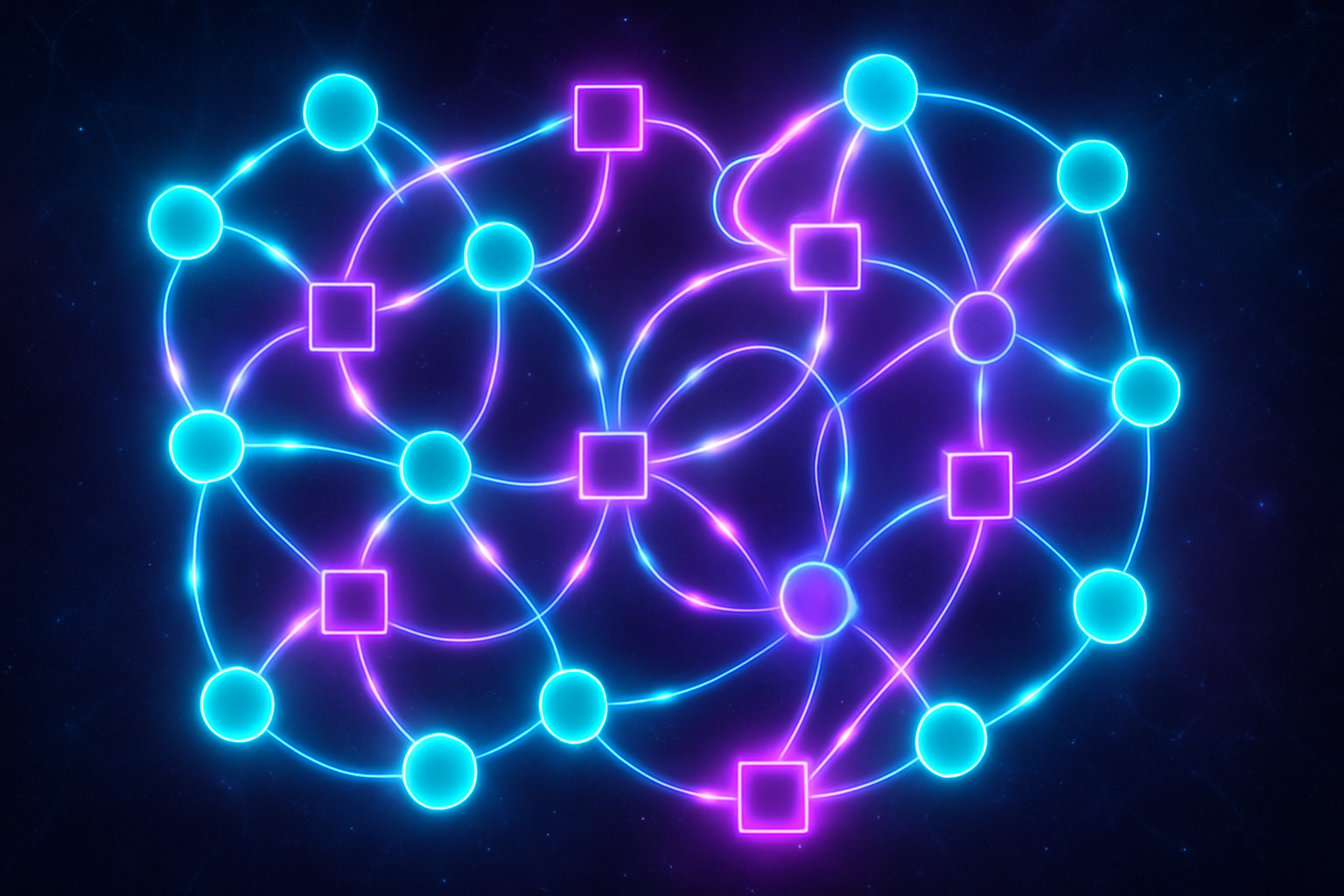
Factor Graphs: Representing Structure as Geometry

A factor graph is a way of visualizing and computing with probabilistic models. It makes explicit which variables depend on which other variables, turning the abstract mathematics of joint probability distributions into something that looks like a diagram of nodes and edges.

There are two types of nodes:

Variable nodes (drawn as circles) represent random variables—hidden states, observations, actions. Each variable node holds a belief distribution over the possible values that variable might take.

Factor nodes (drawn as squares) represent probabilistic relationships between variables. Each factor node encodes a local probability table or function that specifies how its connected variables relate to each other.

Edges connect variable nodes to factor nodes, indicating that a particular variable participates in a particular probabilistic relationship. Crucially, edges only exist where there are direct dependencies. If two variables are conditionally independent given others, there's no edge between them, and the factor graph reflects this by keeping them in separate parts of the graph.

Consider a simple active inference model: an agent observes the world (O), which depends on hidden states (S), which depend on actions (A) the agent takes. This decomposes into factors:

• A factor connecting observations to states: P(O|S)
• A factor connecting states across time: P(S_t | S_{t-1}, A_{t-1})
• A factor representing prior beliefs: P(S_0)

Each factor is local—it only "knows about" the variables it directly connects. The factor P(O|S) doesn't care about actions. The transition factor P(S_t | S_{t-1}, A_{t-1}) doesn't care about observations. This locality is everything.

Factor graphs aren't just a visualization tool. They're a computational architecture. The structure of the graph determines how inference proceeds. Information flows along edges. Beliefs update through local computations at nodes. Complex global inference problems decompose into many small local calculations.

This is how the brain might work—not as a centralized processor computing full joint distributions, but as a distributed network where local circuits pass messages to their neighbors, collectively converging on coherent global beliefs without any single region needing to represent the full state of the world.

In active inference terms, factor graphs are the geometry of inference made literal. The graph's structure encodes the Markov blanket structure of the system—which variables shield which others from direct influence.

The Message Passing Protocol: Local Updates, Global Coherence

Here's the core insight: instead of computing the full joint probability distribution over all variables, we can pass messages between nodes in the factor graph. Each message is a small probability distribution summarizing what one node wants to tell its neighbor about the values that neighbor should consider likely.

The algorithm alternates between two types of updates:

Variable-to-factor messages: A variable node collects all messages it has received from its neighboring factors (except the one it's about to send to), multiplies them together, and sends the result to a factor node. This message says, "Given everything else I've learned, here's my current belief about my value."

Factor-to-variable messages: A factor node computes a message to a variable by marginalizing its local probability table over all other variables connected to it, weighted by the messages it has received from those variables. This message says, "Given the values my other neighbors are reporting, here's what I think you should believe."

Each message is a function of only the messages a node has received from its immediate neighbors. No node needs to know the full graph structure. No node needs to store beliefs about distant variables. Everything is local computation and local communication.

Yet through iterated message exchanges, something remarkable happens: beliefs converge. After several rounds of passing messages back and forth, each variable node's belief distribution approximates the true marginal posterior distribution it would have under exact Bayesian inference. Local computations produce global coherence.

This is belief propagation, and on certain graph structures—trees, where there are no loops—it's not just approximate. It's exact. On tree-structured graphs, belief propagation is guaranteed to converge to the true marginals after a finite number of message passes. The local becomes global. The distributed becomes coordinated.

Real-world models aren't usually trees—they have loops, cycles, dependencies that fold back on themselves. When belief propagation runs on graphs with cycles, it becomes loopy belief propagation, an approximation algorithm that isn't guaranteed to converge but works shockingly well in practice.

Why does loopy belief propagation work at all? Because even on cyclic graphs, messages carry useful information about correlations between variables. The algorithm performs something like iterative refinement—each pass through the graph improves the approximation, even if it never reaches perfect exactness. For active inference agents that need fast approximate answers rather than slow perfect ones, this tradeoff is ideal.

The computational cost of message passing scales linearly with the number of edges in the graph and the number of iterations. This is vastly better than the exponential scaling of exact inference. A model that would take trillions of operations to solve exactly might converge to a good approximation in dozens of message passes.

Variational Message Passing: Minimizing Free Energy Through Messages

Active inference doesn't just perform Bayesian inference—it minimizes variational free energy. This requires a variant of message passing that explicitly optimizes a variational objective.

Standard belief propagation finds marginals. Variational message passing finds an approximate posterior distribution that minimizes the difference between that approximation and the true posterior, measured by KL divergence. In the free energy principle's framing, this is equivalent to minimizing surprise, or equivalently, maximizing evidence lower bound (ELBO).

Variational message passing works by assuming the posterior factorizes across some partition of variables—typically a mean-field approximation where each variable's posterior is independent of the others. This is a strong assumption (and usually wrong), but it makes inference tractable.

The algorithm iterates through variables, updating each one's posterior by fixing all others and minimizing the contribution to free energy from that variable. Messages between variables now carry natural parameters of exponential family distributions—sufficient statistics that summarize beliefs without requiring full distributions to be passed around.

For Gaussian beliefs (common in continuous-state active inference), messages become means and precisions. For categorical beliefs (common in discrete-state models like Markov decision processes), messages become log probability vectors. The updates become coordinate ascent on the ELBO—each variable climbs toward lower free energy given current beliefs about everything else.

This is exactly the algorithm that powers RxInfer.jl, one of the leading active inference software packages. It represents generative models as factor graphs, translates free energy minimization into variational message passing schedules, and compiles the result into efficient inference code. You specify the model structure; the package figures out which messages to pass in which order.

The connection to the free energy principle is direct. Each message update corresponds to a prediction error minimization step. Variable nodes are trying to reconcile top-down predictions (messages from factors representing model structure) with bottom-up evidence (messages from factors representing observations). The fixed point of message passing is the point where prediction errors are minimized—where the agent's beliefs are as coherent with its observations and model as possible.

In neuroscience terms, this is predictive coding implemented as message passing. Higher levels in a cortical hierarchy send predictions down; lower levels send prediction errors up. Each layer updates its beliefs to minimize the mismatch between predictions and inputs. The brain is a factor graph, and attention is the schedule determining which messages get computed when.

Why This Matters: From Math to Metal

Message passing isn't just a computational trick—it's a theory of how biological and artificial agents actually implement inference. The fact that efficient inference on structured probabilistic models looks like local message passing between nodes is not a coincidence. It's a constraint that shapes both brain architecture and AI systems.

Consider what this means for robotics. A robot using active inference needs to infer the state of its joints, the position of objects, the intentions of nearby humans, the stability of its footing—dozens or hundreds of variables, updated in real time at 30+ Hz. Without message passing, this is impossible. With it, the inference problem decomposes. Each subsystem handles local inference; global coherence emerges from message exchanges.

Consider what this means for neuroscience. The brain doesn't have a central inference engine. It has local circuits, each computing with only local information, passing activity patterns to neighbors. If belief propagation describes how these local updates produce coherent perception, that would explain why the brain's architecture—hierarchical, sparsely connected, with recurrent loops—looks exactly like the structure that makes message passing efficient.

The algorithms running in RxInfer and PyMDP aren't simulations of active inference—they are active inference, implemented through the same message passing principles that likely govern neural computation. When you program an agent with RxInfer, you're not specifying low-level operations. You're specifying a generative model, and the package compiles it into a message passing schedule—just as evolution might have compiled the brain's connectivity into an inference machine through natural selection.

This is also why precision-weighting matters so much in active inference. Precision determines how much weight to give different messages. A high-precision observation node sends strong messages—"Trust me, this is what you observed." A low-precision observation sends weak messages—"This is noisy, take it with a grain of salt." Modulating precision is how the brain implements attention: turning up gain on relevant messages, turning down gain on irrelevant ones.

Schizophrenia, in this framework, might involve aberrant precision. If sensory messages arrive with too much precision, hallucinations emerge—priors can't override observations. If priors arrive with too much precision, delusions persist—evidence can't update beliefs. The message passing framework makes these hypotheses testable. You can build agents with different precision schedules and see which behaviors emerge.

Implementation: Seeing Message Passing in Code

Here's what variational message passing looks like in RxInfer.jl, stripped to essentials:

@model function simple_agent(observations)
    # Prior over initial state
    s_0 ~ Normal(0.0, 1.0)

    # Transition dynamics
    s ~ Normal(s_0, 0.5)

    # Observation model
    o ~ Normal(s, 0.1)

    # Condition on actual observations
    o .= observations
end

# Infer hidden state
result = infer(
    model = simple_agent(observations = [1.0, 1.2, 1.1]),
    returnvars = (s = KeepLast(),)
)

What happens under the hood:

1. RxInfer converts the model into a factor graph with variable nodes (s_0, s, o) and factor nodes (Normal distributions connecting them).

2. It determines a message passing schedule—which messages to compute in which order to minimize free energy.

3. It iterates through the schedule, passing messages between nodes until beliefs converge.

4. The final belief about s emerges from the fixed point of these local computations—no explicit global optimization, just messages that collectively minimize surprise.

In PyMDP (the Python implementation for discrete active inference), the same principles apply but for categorical distributions. Agents represent beliefs as probability vectors over discrete states. Messages become matrix multiplications and normalizations. The math is different; the architecture is identical.

Both frameworks let you specify models declaratively—you say what the structure is, and the package figures out how to compute with it. This is the power of message passing: the algorithm is model-agnostic. Change the graph structure, and the schedule adapts automatically. Add a new variable, and messages reroute accordingly. The separation between model and inference is clean.

This also means you can debug inference problems by visualizing the factor graph. If beliefs aren't converging, you can trace the message paths, identify bottlenecks, adjust precision parameters. Inference becomes interpretable, not a black box.

Connection to AToM: Messages as Coherence Negotiation

In AToM terms—where meaning equals coherence over time (M = C/T)—message passing is the mechanism by which local subsystems negotiate toward global coherence.

Each message is a proposal: "Here's what I think we should believe about this variable." Each update is an attempt to reconcile conflicting proposals. Convergence is the achievement of a coherent interpretation—a set of beliefs that mutually support each other, that minimize tension between observations and predictions, that hold together across time.

When message passing fails to converge, the system lacks coherence. Beliefs oscillate. Predictions conflict. This is high curvature in AToM's geometry—instability, fragmentation, the inability to settle on a consistent interpretation of the world.

When message passing converges rapidly, the system has high coherence. Beliefs crystallize. Predictions align. This is low curvature—stability, integration, a trajectory through state space that's sustainable over time.

Precision-weighting is the mechanism that controls coherence. High precision enforces coherence—messages insist on agreement. Low precision permits diversity—messages tolerate disagreement. An agent that's too precise becomes rigid, unable to update when the world changes. An agent that's too imprecise becomes chaotic, unable to maintain stable beliefs. The optimal precision schedule balances coherence and flexibility—enough structure to act, enough openness to learn.

This is why trauma disrupts message passing. If precision is chronically misallocated—hyper-vigilance toward threat signals, hypo-vigilance toward safety signals—the inference schedule becomes pathological. Messages from the body saying "You're safe now" get ignored. Messages from memory saying "This is like that time you were hurt" get amplified. Coherence collapses. Meaning fragments.

The therapeutic task, in this framing, is to recalibrate precision—to restore the message passing schedule that allows past and present, body and mind, prediction and observation to negotiate toward coherence. This might involve somatic practices that reweight interoceptive messages, narrative therapy that restructures the factor graph of autobiographical memory, or pharmacological interventions that modulate precision at a neurochemical level.

Message passing, then, isn't just an algorithm. It's a mechanism of meaning-making, the process by which systems construct and maintain coherent interpretations of themselves and their environments.

Further Reading

• Dauwels, J. (2007). "On Variational Message Passing on Factor Graphs." Proceedings of IEEE International Symposium on Information Theory.
• Friston, K., Parr, T., & de Vries, B. (2017). "The graphical brain: Belief propagation and active inference." Network Neuroscience, 1(4), 381-414.
• Loeliger, H. A. (2004). "An introduction to factor graphs." IEEE Signal Processing Magazine, 21(1), 28-41.
• Winn, J., & Bishop, C. M. (2005). "Variational message passing." Journal of Machine Learning Research, 6, 661-694.
• Yedidia, J. S., Freeman, W. T., & Weiss, Y. (2003). "Understanding belief propagation and its generalizations." Exploring Artificial Intelligence in the New Millennium, 8, 236-239.

This is Part 4 of the Active Inference Applied series, exploring how active inference moves from theory to implementation.

Previous: Expected Free Energy: The Objective Function That Plans
Next: PyMDP and RxInfer: The Active Inference Software Stack