The Chain Rule in Multiple Variables

The Chain Rule in Multiple Variables | Ideasthesia

In single-variable calculus, the chain rule is d/dx[f(g(x))] = f'(g(x)) · g'(x). You differentiate the outer function, evaluate it at the inner function, then multiply by the derivative of the inner function.

In multivariable calculus, the chain rule handles much more complex dependency structures: functions that depend on multiple variables, which themselves depend on other variables, forming networks of dependencies.

This is the mathematical machinery of backpropagation in neural networks, sensitivity analysis in engineering, thermodynamic relations in physics—anywhere you need to track how changes propagate through systems of interdependent variables.

The multivariable chain rule isn't just "the single-variable chain rule with more symbols." It's a systematic way of computing derivatives through dependency graphs, using tree diagrams or matrices to organize the calculation.

The Basic Setup: Composition with Multiple Inputs

The simplest multivariable chain rule handles a composition where the outer function has multiple inputs, but those inputs depend on a single variable.

Suppose z = f(x, y), and both x and y depend on a single variable t:

x = x(t)
y = y(t)

Then z is indirectly a function of t: z = f(x(t), y(t)).

The question: what is dz/dt?

The chain rule answer:

dz/dt = (∂f/∂x)(dx/dt) + (∂f/∂y)(dy/dt)

In words: the rate of change of z with respect to t is the sum of two contributions:

How z changes with x (∂f/∂x), weighted by how x changes with t (dx/dt)
How z changes with y (∂f/∂y), weighted by how y changes with t (dy/dt)

This is additive composition of rates: changes in x and y both contribute to changes in z, and you add their effects.

Example: z = x² + y², where x = cos(t) and y = sin(t).

Direct approach: substitute to get z = cos²(t) + sin²(t) = 1, so dz/dt = 0.

Chain rule approach:

∂z/∂x = 2x, ∂z/∂y = 2y
dx/dt = -sin(t), dy/dt = cos(t)
dz/dt = 2x(-sin(t)) + 2y(cos(t)) = 2cos(t)(-sin(t)) + 2sin(t)(cos(t)) = -2cos(t)sin(t) + 2sin(t)cos(t) = 0

The chain rule confirms: z is constant along the path (x(t), y(t)), so dz/dt = 0.

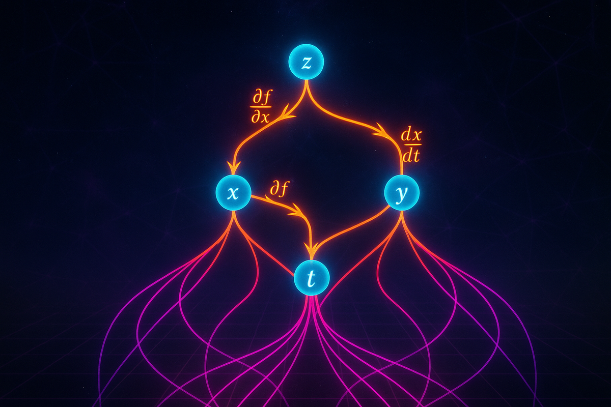
Tree Diagrams: Visualizing Dependencies

To organize multivariable chain rule calculations, use a tree diagram showing the dependency structure.

For z = f(x, y) with x = x(t), y = y(t):

To find dz/dt, trace all paths from z to t:

Path through x: multiply ∂z/∂x and dx/dt
Path through y: multiply ∂z/∂y and dy/dt
Sum the contributions

This tree method scales to arbitrarily complex dependency structures.

More complex example: w = f(x, y, z) where:

x = x(s, t)
y = y(s, t)
z = z(s, t)

To find ∂w/∂s:

Trace paths from w to s:

Through x: ∂w/∂x · ∂x/∂s
Through y: ∂w/∂y · ∂y/∂s
Through z: ∂w/∂z · ∂z/∂s

Sum them:

∂w/∂s = (∂w/∂x)(∂x/∂s) + (∂w/∂y)(∂y/∂s) + (∂w/∂z)(∂z/∂s)

The tree diagram makes the structure obvious: every intermediate variable contributes a term.

The General Multivariable Chain Rule

If z = f(x₁, x₂, ..., xₙ) and each xᵢ depends on variables t₁, t₂, ..., t_m, then:

∂z/∂t_j = Σᵢ (∂f/∂xᵢ)(∂xᵢ/∂t_j)

You sum over all intermediate variables xᵢ, multiplying the partial derivative with respect to xᵢ by the partial derivative of xᵢ with respect to t_j.

This is the matrix form of the chain rule:

∇f (the gradient of f) is a row vector: (∂f/∂x₁, ∂f/∂x₂, ..., ∂f/∂xₙ)

J (the Jacobian of x with respect to t) is an n×m matrix:

J = [∂xᵢ/∂t_j]

The gradient of z with respect to t is:

∇z = ∇f · J

This matrix multiplication automatically sums the contributions from all paths through the dependency graph.

Implicit Differentiation as a Chain Rule Application

Implicit differentiation—finding dy/dx when x and y are related by an equation F(x, y) = 0—is a chain rule application.

Consider F(x, y) = 0. If y is implicitly a function of x, then F(x, y(x)) = 0 for all x.

Differentiate both sides with respect to x using the chain rule:

dF/dx = (∂F/∂x)(dx/dx) + (∂F/∂y)(dy/dx) = ∂F/∂x + (∂F/∂y)(dy/dx) = 0

Solve for dy/dx:

dy/dx = -(∂F/∂x) / (∂F/∂y)

Example: x² + y² = 25 (a circle).

F(x, y) = x² + y² - 25

∂F/∂x = 2x, ∂F/∂y = 2y

dy/dx = -2x / 2y = -x/y

This matches what you'd get by differentiating x² + y² = 25 directly and solving for dy/dx.

The chain rule formalism makes implicit differentiation mechanical: compute partial derivatives of F, plug into the formula.

The Chain Rule and Coordinate Transformations

When you change coordinates (say, from Cartesian to polar), the chain rule tells you how derivatives transform.

Suppose f is a function of x and y, and you want to express it in polar coordinates (r, θ), where:

x = r cos(θ)
y = r sin(θ)

To find ∂f/∂r, use the chain rule:

∂f/∂r = (∂f/∂x)(∂x/∂r) + (∂f/∂y)(∂y/∂r)

Compute:

∂x/∂r = cos(θ), ∂y/∂r = sin(θ)

So:

∂f/∂r = (∂f/∂x)cos(θ) + (∂f/∂y)sin(θ)

Similarly for ∂f/∂θ:

∂f/∂θ = (∂f/∂x)(∂x/∂θ) + (∂f/∂y)(∂y/∂θ)

where ∂x/∂θ = -r sin(θ), ∂y/∂θ = r cos(θ), giving:

∂f/∂θ = (∂f/∂x)(-r sin(θ)) + (∂f/∂y)(r cos(θ))

These formulas let you convert between coordinate systems without explicitly substituting and re-differentiating.

This is how you derive the gradient in polar coordinates or any other curvilinear system: apply the chain rule to relate derivatives in the new coordinates to derivatives in Cartesian coordinates.

Backpropagation: The Chain Rule in Neural Networks

In deep learning, a neural network is a composition of many functions:

y = f_L(f_{L-1}(...f_2(f_1(x))))

where each f_i is a layer (linear transformation plus activation).

To train the network, you need to compute the gradient of a loss function L(y) with respect to the parameters in each layer.

This is done via backpropagation, which is just the multivariable chain rule applied recursively:

∂L/∂w_i = (∂L/∂y)(∂y/∂f_L)(∂f_L/∂f_{L-1})...(∂f_{i+1}/∂f_i)(∂f_i/∂w_i)

You start at the output (∂L/∂y) and propagate gradients backward through the network, multiplying by the derivative of each layer.

The chain rule organizes the computation: each layer computes its local derivative (∂f_i/∂w_i) and passes gradients to the previous layer. The global gradient is the product of all these local derivatives.

Without the multivariable chain rule, training deep networks would be intractable. It's the mathematical engine of modern AI.

The Jacobian Matrix: Generalizing the Derivative

For single-variable functions, the derivative is a number. For multivariable scalar functions, the derivative is the gradient (a vector).

But what if the function is vector-valued? What if f: ℝⁿ → ℝᵐ takes n inputs and produces m outputs?

The derivative is the Jacobian matrix J, an m×n matrix of partial derivatives:

J_ij = ∂f_i / ∂x_j

Each row is the gradient of one component function f_i.

Example: f(x, y) = (x²y, xy², x + y)

This maps ℝ² → ℝ³. The Jacobian is:

J = [∂f₁/∂x ∂f₁/∂y] [2xy x² ] [∂f₂/∂x ∂f₂/∂y] = [y² 2xy ] [∂f₃/∂x ∂f₃/∂y] [1 1 ]

The Jacobian generalizes the derivative to vector-valued functions. When you compose vector-valued functions, you multiply their Jacobians—this is the matrix form of the chain rule.

If g: ℝᵏ → ℝⁿ and f: ℝⁿ → ℝᵐ, then the composition h = f ∘ g has Jacobian:

J_h = J_f · J_g

This is exactly the multivariable chain rule in matrix form.

Higher-Order Chain Rules

Just as you can have second derivatives, you can apply the chain rule to second derivatives.

If z = f(x, y) and x, y depend on t, then:

d²z/dt² = d/dt[dz/dt]

Expand dz/dt = (∂f/∂x)(dx/dt) + (∂f/∂y)(dy/dt), then differentiate again using the product rule and chain rule:

d²z/dt² = (∂²f/∂x²)(dx/dt)² + 2(∂²f/∂x∂y)(dx/dt)(dy/dt) + (∂²f/∂y²)(dy/dt)² + (∂f/∂x)(d²x/dt²) + (∂f/∂y)(d²y/dt²)

This gets complicated quickly, involving second partial derivatives (the Hessian matrix) and second derivatives of the path variables.

The takeaway: higher-order chain rules exist and follow the same pattern (differentiate, apply product and chain rules), but the notation becomes dense.

Thermodynamic Example: Maxwell Relations

In thermodynamics, energy U is a function of entropy S and volume V: U = U(S, V).

But S and V might depend on temperature T and pressure P: S = S(T, P), V = V(T, P).

To find ∂U/∂T at constant P, use the chain rule:

(∂U/∂T)_P = (∂U/∂S)(∂S/∂T)_P + (∂U/∂V)(∂V/∂T)_P

This expresses how internal energy changes with temperature in terms of how energy depends on entropy and volume, combined with how entropy and volume respond to temperature.

Maxwell relations arise from the equality of mixed partial derivatives (∂²U/∂S∂V = ∂²U/∂V∂S), applied via the chain rule to thermodynamic potentials.

The chain rule is how you navigate between different choices of independent variables in thermodynamics—a subject notorious for having many equivalent formulations.

Chain Rule for Parametric Surfaces

If a surface is parametrized by r(u, v) = (x(u, v), y(u, v), z(u, v)), and you have a function f(x, y, z) defined on the surface, the chain rule gives you derivatives with respect to the parameters u and v:

∂f/∂u = (∂f/∂x)(∂x/∂u) + (∂f/∂y)(∂y/∂u) + (∂f/∂z)(∂z/∂u)

∂f/∂v = (∂f/∂x)(∂x/∂v) + (∂f/∂y)(∂y/∂v) + (∂f/∂z)(∂z/∂v)

In vector notation:

∂f/∂u = ∇f · (∂r/∂u)

∂f/∂v = ∇f · (∂r/∂v)

The tangent vectors ∂r/∂u and ∂r/∂v span the tangent plane to the surface, and the chain rule projects the gradient onto these tangent directions.

This is how you compute rates of change along surfaces: use the chain rule to connect the gradient (which lives in ambient space) to tangent vectors (which live on the surface).

When the Chain Rule Fails

The multivariable chain rule requires differentiability of the composed functions.

If f is not differentiable at a point, or if x(t) or y(t) aren't differentiable, the chain rule doesn't apply.

Also, the chain rule assumes the functions are genuinely functions—single-valued. If you have multivalued relations (like square roots or inverse trig functions with multiple branches), you need to be careful about which branch you're on.

For continuous but non-differentiable functions (like f(x, y) = |x| + |y|), you can't use the chain rule through the non-differentiable points.

Computational Strategy: Always Draw the Tree

When faced with a multivariable chain rule problem, the best strategy is:

Draw the dependency tree showing which variables depend on which.
Identify all paths from the output variable to the variable you're differentiating with respect to.
Multiply derivatives along each path (partial derivatives for each step).
Sum all path contributions.

This method works for any dependency structure, no matter how complex.

Example: w = f(u, v), where u = g(x, y) and v = h(x, y). Find ∂w/∂x.

Tree:

Paths from w to x:

w → u → x: multiply ∂w/∂u and ∂u/∂x
w → v → x: multiply ∂w/∂v and ∂v/∂x

Sum:

∂w/∂x = (∂w/∂u)(∂u/∂x) + (∂w/∂v)(∂v/∂x)

The tree makes it trivial to get the right formula.

The Chain Rule and Gradient Descent

In gradient descent, you update parameters by stepping in the direction of the negative gradient.

When the loss function is a composition (as in neural networks), you need the chain rule to compute the gradient.

For L(f(θ)), where θ are parameters and f is a model:

∇_θ L = (dL/df) · ∇_θ f

The gradient with respect to parameters is the gradient of the loss with respect to the model output, times the Jacobian of the model with respect to parameters.

This is how automatic differentiation libraries (like PyTorch, TensorFlow) work: they build a computation graph (dependency tree), then apply the chain rule backward from the loss to all parameters.

The multivariable chain rule is the algorithmic backbone of modern optimization.

The total derivative generalizes the chain rule to describe how a function changes when all its variables change.

For z = f(x, y), the total differential is:

dz = (∂f/∂x)dx + (∂f/∂y)dy

This says: a small change dz in z is approximately the sum of (∂f/∂x)dx (contribution from change in x) and (∂f/∂y)dy (contribution from change in y).

If x and y are functions of t, then dx = (dx/dt)dt and dy = (dy/dt)dt, so:

dz = (∂f/∂x)(dx/dt)dt + (∂f/∂y)(dy/dt)dt

Divide by dt:

dz/dt = (∂f/∂x)(dx/dt) + (∂f/∂y)(dy/dt)

This is the chain rule again. The total differential formalism is an alternative notation that emphasizes infinitesimal changes.

The Conceptual Core: Derivatives Compose Multiplicatively

The fundamental idea: when functions compose, their derivatives multiply (or, in the multivariable case, sum over multiplication along paths).

This is true whether you're in one dimension or many. The multivariable chain rule just tracks multiple paths and sums their contributions.

Mathematically, this reflects the fact that the derivative is a linear approximation, and linear maps compose via matrix multiplication (which generalizes scalar multiplication).

Conceptually, it reflects how change propagates through systems: if A affects B, and B affects C, then A's effect on C is mediated by A's effect on B and B's effect on C.

The chain rule is the mathematical formalization of indirect causation.

What's Next

We've completed the toolkit for differentiation in multiple variables:

Partial derivatives for change along axes
Gradients for steepest ascent
Directional derivatives for change in arbitrary directions
The chain rule for change through compositions

Now we shift to integration: accumulating quantities over regions and volumes.

First up: double integrals, which let you integrate over two-dimensional regions to compute areas, volumes, masses, and other aggregated quantities.

Then triple integrals for three-dimensional volumes.

Then the Jacobian (again, but for integrals this time), which describes how to change coordinates when integrating.

Finally, Lagrange multipliers for constrained optimization—finding maxima and minima subject to constraints, using the gradient as the key tool.

The chain rule bridges differentiation and integration, optimization and analysis. It's the connective tissue of multivariable calculus.

With it mastered, we're ready to integrate.

Part 5 of the Multivariable Calculus series.

Previous: Directional Derivatives: Rates of Change in Any Direction Next: Double Integrals: Integrating Over Regions