The Normal Distribution: The Bell Curve and Why It Appears Everywhere

Heights. IQ scores. Measurement errors. Stock returns. Blood pressure. Manufacturing tolerances. Test grades.

All approximately normal. All follow the bell curve.

This isn't coincidence. There's a deep mathematical reason—the Central Limit Theorem—that explains why so many phenomena produce normal distributions.

The Definition

The normal distribution with mean μ and variance σ² has probability density:

f(x) = (1 / √(2πσ²)) × exp(-(x-μ)² / 2σ²)

The standard normal has μ = 0, σ = 1:

φ(z) = (1 / √(2π)) × exp(-z²/2)

Any normal can be standardized: if X ~ Normal(μ, σ²), then Z = (X - μ)/σ ~ Normal(0, 1).

Properties

Symmetry: The normal distribution is symmetric around μ.

Mean = Mode = Median: All three measures of center coincide.

Probabilities:

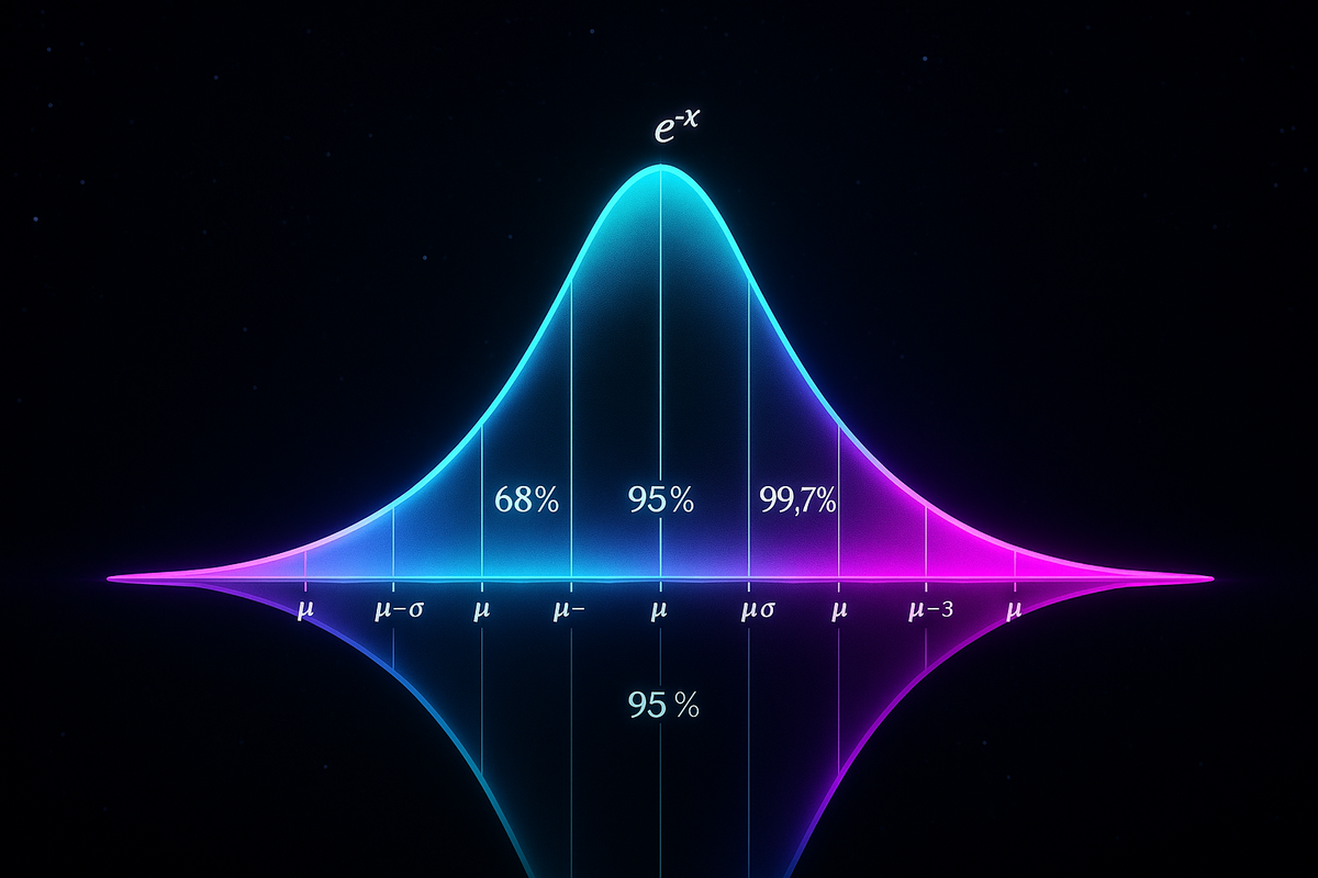
• 68.3% within 1σ of μ
• 95.4% within 2σ
• 99.7% within 3σ

Tails: The tails decay exponentially fast. Extreme values are very rare.

Sum of Normals: If X ~ Normal(μ₁, σ₁²) and Y ~ Normal(μ₂, σ₂²) are independent, then X + Y ~ Normal(μ₁ + μ₂, σ₁² + σ₂²).

Linear Transformation: If X is normal, aX + b is normal.

The Bell Curve Shape

The equation e^(-x²) creates the characteristic bell.

Near x = 0, e^(-x²) ≈ 1. As x grows, e^(-x²) plummets. At x = 2, it's already e^(-4) ≈ 0.018.

The σ parameter controls width. Large σ means a wide, short bell. Small σ means a narrow, tall bell. The total area is always 1.

Why Normal Appears Everywhere

The Central Limit Theorem (CLT):

The sum of many independent random variables is approximately normal—regardless of what distribution each individual variable has.

Example: Height.

Your height is influenced by thousands of genes, each contributing a small effect, plus environmental factors. The sum of many small independent contributions → approximately normal.

Example: Measurement error.

Many tiny disturbances combine to produce measurement error. The sum → approximately normal.

Example: Aggregate outcomes.

Test scores (sum of many question performances), daily returns (aggregate of many trades), biological measurements (sum of many cellular processes)—all sums of many factors, all approximately normal.

The CLT is profound: it explains why the same distribution keeps appearing in completely unrelated contexts.

The Standard Normal Table

For the standard normal, we often need P(Z ≤ z), denoted Φ(z).

This can't be computed in closed form—it requires numerical methods or tables.

Key values:

• Φ(0) = 0.5
• Φ(1) ≈ 0.841
• Φ(1.645) ≈ 0.95
• Φ(1.96) ≈ 0.975
• Φ(2.576) ≈ 0.995

For non-standard normals: P(X ≤ x) = Φ((x - μ)/σ)

Applications

Quality Control:

A manufacturing process produces parts with normally distributed dimensions. Set tolerance limits at μ ± 3σ and 99.7% of parts will be acceptable.

Finance:

Stock returns are modeled (imperfectly) as normal. This underlies Black-Scholes options pricing and Value at Risk calculations.

Testing:

z-scores and t-tests assume normally distributed data. The normal distribution is the backbone of frequentist statistics.

Errors:

Maximum likelihood estimation with normal errors leads to least squares regression. Assume normal errors, minimize squared errors.

Not Everything Is Normal

The normal distribution assumes:

• Finite variance
• Symmetric distribution
• Independence or weak dependence

Violations lead to non-normal distributions:

Power laws: Wealth, city sizes, word frequencies. Heavy tails, not normal.

Extreme events: Financial crashes, earthquakes. Fat tails—more extreme events than normal predicts.

Bounded variables: Percentages, probabilities. Truncated, not normal.

Discrete counts: Number of emails, accidents. Poisson or binomial, not normal.

Log-normal: Income, particle sizes. Logarithm is normal, not the variable itself.

Assuming normality when it doesn't apply leads to underestimating extreme risks. This was a factor in the 2008 financial crisis.

The Normal as Limit

Several distributions become normal as parameters grow:

Binomial(n, p) → Normal(np, np(1-p)) as n → ∞

For large n, the binomial approximates a normal with matching mean and variance.

Poisson(λ) → Normal(λ, λ) as λ → ∞

Large-rate Poisson is approximately normal.

Student's t → Standard Normal as degrees of freedom → ∞

The t-distribution has heavier tails than normal, but converges to normal with many observations.

These approximations are all manifestations of the CLT.

Multivariate Normal

In multiple dimensions, the normal distribution generalizes.

A random vector (X₁, X₂, ..., Xₙ) is multivariate normal if every linear combination is univariate normal.

Characterized by:

• Mean vector μ
• Covariance matrix Σ

The covariance matrix generalizes variance. Diagonal entries are variances; off-diagonal entries are covariances.

Contours: In 2D, constant-probability contours are ellipses. The shape depends on variances and correlation.

Multivariate normal is fundamental to:

• Principal component analysis
• Gaussian processes
• Bayesian inference
• Factor analysis

Maximum Entropy

The normal distribution maximizes entropy among distributions with fixed mean and variance.

If you know only the mean and variance of a continuous random variable, the most "uncertain" (least presumptuous) distribution is normal.

This provides a justification for using normal distributions as default assumptions.

Historical Note

The normal distribution was discovered multiple times:

• De Moivre (1733): as approximation to binomial
• Laplace (1774): independently, for error theory
• Gauss (1809): for astronomical observations

It's called "Gaussian" in scientific contexts, "normal" in statistical contexts. The terminology "normal" comes from the 19th century belief that this distribution was the norm for natural phenomena.

The mathematical significance was fully understood only with the Central Limit Theorem, proved rigorously in the 20th century.

The Pebble

The normal distribution isn't special because we chose it. It's special because mathematics chose it.

When many small effects combine, the result is normal—regardless of what the individual effects look like. This emergence of order from randomness is remarkable.

The bell curve is nature's favorite shape for continuous uncertainty. Understanding it is understanding a deep truth about how randomness behaves in aggregate.

This is Part 8 of the Probability series. Next: "Probability Distributions: The Complete Catalog."

Part 8 of the Probability series.

Previous: Variance and Standard Deviation: Measuring Spread Next: Common Distributions: Binomial Poisson and Beyond