Optimization: Finding Maxima and Minima with Derivatives

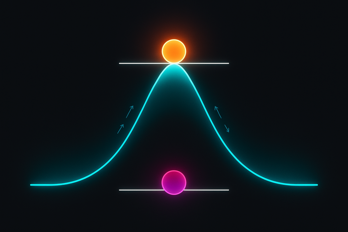
At a peak or valley, the slope is zero.

That's the key insight. When a function reaches its highest or lowest point (locally), it's momentarily flat. The tangent line is horizontal. The derivative equals zero.

Here's the unlock: to find maxima and minima, find where the derivative is zero. These are the critical points — the candidates for peaks and valleys. Then check which ones are actually maxima, which are minima, and which are neither.

The derivative doesn't just measure change. It locates the turning points.

Why Derivative = 0 at Extrema

At a local maximum:

• To the left, the function is increasing (f' > 0)
• To the right, the function is decreasing (f' < 0)
• At the peak, it's neither — f' = 0

At a local minimum:

• To the left, the function is decreasing (f' < 0)
• To the right, the function is increasing (f' > 0)
• At the valley, it's neither — f' = 0

The transition from positive to negative slope (or vice versa) passes through zero.

Critical Points

A critical point is where f'(x) = 0 or f'(x) is undefined.

Finding critical points:

1. Compute f'(x)
2. Set f'(x) = 0 and solve
3. Also note where f'(x) doesn't exist

Not every critical point is a max or min. Some are inflection points (where concavity changes but there's no extreme value).

Example: f(x) = x³ - 3x + 1

Find f'(x): f'(x) = 3x² - 3 = 3(x² - 1) = 3(x-1)(x+1)

Set f'(x) = 0: x = 1 or x = -1

These are the critical points.

Evaluate f at critical points: f(-1) = (-1)³ - 3(-1) + 1 = -1 + 3 + 1 = 3 f(1) = (1)³ - 3(1) + 1 = 1 - 3 + 1 = -1

So (-1, 3) and (1, -1) are critical points.

First Derivative Test

Check the sign of f' around each critical point:

At x = -1:

• f'(-2) = 3(4-1) = 9 > 0 (increasing before)
• f'(0) = 3(0-1) = -3 < 0 (decreasing after)
• Going from + to - means local maximum at x = -1

At x = 1:

• f'(0) = -3 < 0 (decreasing before)
• f'(2) = 3(4-1) = 9 > 0 (increasing after)
• Going from - to + means local minimum at x = 1

Second Derivative Test

If f'(c) = 0 and:

• f''(c) > 0: the curve is concave up, so local minimum
• f''(c) < 0: the curve is concave down, so local maximum
• f''(c) = 0: test is inconclusive (use first derivative test)

For f(x) = x³ - 3x + 1: f''(x) = 6x

At x = -1: f''(-1) = -6 < 0 → local maximum ✓ At x = 1: f''(1) = 6 > 0 → local minimum ✓

Absolute (Global) Extrema

On a closed interval [a, b], a continuous function must attain an absolute max and min.

Candidates:

1. Critical points inside (a, b)
2. Endpoints a and b

Evaluate f at all candidates. The largest is the absolute max; the smallest is the absolute min.

Example: Absolute Extrema on [0, 3]

Find the absolute max and min of f(x) = x³ - 3x + 1 on [0, 3].

Critical point in (0, 3): x = 1 (found earlier)

Evaluate at candidates:

• f(0) = 0 - 0 + 1 = 1
• f(1) = 1 - 3 + 1 = -1
• f(3) = 27 - 9 + 1 = 19

Absolute maximum: 19 at x = 3 Absolute minimum: -1 at x = 1

Applied Optimization

The procedure:

1. Draw and label: Identify variables and constraints
2. Write the objective function: What are you maximizing/minimizing?
3. Use constraints: Reduce to one variable if possible
4. Differentiate: Find critical points
5. Check: Verify it's the right type of extremum
6. Answer the question: Give the final answer in context

Example: Maximizing Area

A farmer has 100 m of fencing to enclose a rectangular area against a barn (which forms one side). What dimensions maximize the enclosed area?

Variables: Let x = length perpendicular to barn, y = length parallel to barn.

Constraint: 2x + y = 100 (fencing), so y = 100 - 2x.

Objective: A = xy = x(100 - 2x) = 100x - 2x²

Differentiate: A'(x) = 100 - 4x

Critical point: 100 - 4x = 0 → x = 25

Check: A''(x) = -4 < 0, so x = 25 is a maximum.

Dimensions: x = 25 m, y = 100 - 50 = 50 m. Maximum area: A = 25 × 50 = 1250 m².

Example: Minimizing Material

Design a cylindrical can to hold 1 liter (1000 cm³) with minimum surface area.

Variables: r = radius, h = height.

Constraint: V = πr²h = 1000, so h = 1000/(πr²).

Objective: S = 2πr² + 2πrh (top + bottom + side)

Substitute h: S = 2πr² + 2πr · 1000/(πr²) = 2πr² + 2000/r

Differentiate: dS/dr = 4πr - 2000/r²

Critical point: 4πr = 2000/r², so r³ = 500/π, r = ∛(500/π) ≈ 5.42 cm.

Height: h = 1000/(π · 5.42²) ≈ 10.84 cm.

Note: h ≈ 2r. The optimal can has height equal to its diameter.

Constraints and Lagrange Multipliers

When optimizing with constraints that can't be eliminated easily, use Lagrange multipliers (multivariable calculus topic):

Optimize f(x,y) subject to g(x,y) = 0 by solving: ∇f = λ∇g and g(x,y) = 0

The Core Insight

Derivatives locate extrema because extrema have zero slope.

At a peak, you're not going up or down — you're momentarily flat. Setting f'(x) = 0 finds those flat moments. The second derivative (or sign analysis) tells you whether it's a hilltop or a valley floor.

Optimization is the practical payoff of differential calculus. You can find the best dimensions, the minimum cost, the maximum profit — all by finding where the rate of change hits zero.

The universe optimizes constantly. Derivatives show you where.

Part 11 of the Calculus Derivatives series.

Previous: Derivatives of Trigonometric Functions: Why d/dx(sin x) = cos x Next: Synthesis: The Derivative as the Language of Rates