Parametric Equations: Two Functions One Curve

A circle.

In standard form: x² + y² = 1.

But how do you trace the circle? How do you describe a point moving around it?

Parametric equations.

x = cos(t) y = sin(t)

As t goes from 0 to 2π, the point (x, y) traces the full circle.

Parametric equations describe motion. The parameter—usually t—represents time. The equations describe position as a function of time.

The Unlock: Describing Curves That Move

Most functions are written y = f(x). For each x, there's one y.

But some curves loop, spiral, or backtrack. A vertical line test fails. You can't write them as y = f(x).

Parametric equations solve this.

Instead of y = f(x), you write: x = f(t) y = g(t)

As t varies, you trace a curve in the xy-plane. No restriction on loops or multiple y-values for a single x.

Parametric equations describe curves as paths, not as graphs of functions.

The Parameter

The variable t is the parameter. It's independent of x and y.

Often, t represents time. The parametric equations describe position at each moment.

But t doesn't have to be time. It's just a variable that traces the curve.

Example: A circle.

x = cos(t) y = sin(t)

t is the angle (in radians) from the positive x-axis. As t increases, you move counterclockwise around the circle.

Eliminating the Parameter

To convert parametric equations to a standard equation, eliminate the parameter.

Example: x = cos(t), y = sin(t).

Use the identity cos²(t) + sin²(t) = 1.

x² + y² = 1.

This is the equation of a circle.

Example: x = 2t, y = t².

Solve the first equation for t: t = x/2.

Substitute into the second: y = (x/2)² = x²/4.

The curve is a parabola: y = x²/4.

Why Parametric Equations Are More General

Some curves can't be written as y = f(x).

Example: A circle. For most x-values, there are two y-values (top and bottom of the circle).

But in parametric form, it's simple: x = cos(t) y = sin(t)

One equation pair describes the entire circle.

Parametric equations let you describe any curve, no matter how it loops or twists.

Curves That Backtrack

Consider: x = t³ - 3t y = t²

As t varies from -2 to 2, x is not monotonic. The curve backtracks—it moves right, then left, then right again.

This can't be written as y = f(x) because multiple t-values give the same x.

But parametrically, it's straightforward.

The Unit Circle

x = cos(t) y = sin(t) t ∈ [0, 2π]

This is the unit circle, traced counterclockwise starting from (1, 0).

At t = 0: (1, 0). At t = π/2: (0, 1). At t = π: (-1, 0). At t = 3π/2: (0, -1). At t = 2π: back to (1, 0).

This is the most fundamental parametric curve.

Lines in Parametric Form

A line through a point (x₀, y₀) in the direction of a vector (a, b):

x = x₀ + at y = y₀ + bt

As t varies, you trace the entire line.

Example: Line through (1, 2) in the direction (3, -1):

x = 1 + 3t y = 2 - t

At t = 0: (1, 2). At t = 1: (4, 1). At t = -1: (-2, 3).

Parametric form makes it easy to describe lines in any direction.

Ellipses in Parametric Form

x = a cos(t) y = b sin(t)

This traces an ellipse centered at the origin with semi-major axis a and semi-minor axis b.

Example: x = 3 cos(t), y = 2 sin(t).

As t goes from 0 to 2π, you trace the ellipse x²/9 + y²/4 = 1.

Spirals

Parametric equations can describe spirals.

Archimedean spiral: x = t cos(t) y = t sin(t)

The radius increases linearly with t. The curve spirals outward.

Logarithmic spiral: x = e^t cos(t) y = e^t sin(t)

The radius grows exponentially. This spiral appears in shells and galaxies.

Cycloids

A cycloid is the curve traced by a point on the rim of a rolling circle.

Imagine a bicycle wheel rolling along the ground. A pebble stuck to the tire traces a cycloid.

Parametric equations: x = r(t - sin(t)) y = r(1 - cos(t))

where r is the radius of the circle.

The cycloid has arches—it loops up, comes down, touches the ground, and loops up again.

Cycloids have remarkable properties. The brachistochrone curve (fastest descent) is a cycloid. So is the tautochrone curve (equal time to the bottom).

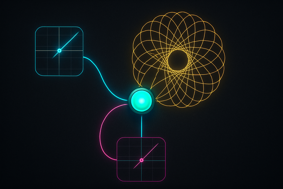
Lissajous Curves

Combine two sine waves with different frequencies:

x = A sin(at + δ) y = B sin(bt)

These are Lissajous curves. They create intricate looping patterns.

Example: x = sin(2t), y = sin(3t).

The curve loops and crosses itself in a symmetric pattern.

Lissajous curves appear in oscilloscopes, signal processing, and music theory.

Parametric Equations for Motion

In physics, parametric equations describe trajectories.

Projectile motion: x = v₀t cos(θ) y = v₀t sin(θ) - (1/2)gt²

v₀ is initial velocity, θ is launch angle, g is gravity.

x(t) describes horizontal position. y(t) describes vertical position.

Eliminating t gives the trajectory as a function of x (a parabola). But the parametric form shows how position changes with time.

Speed and Velocity

For parametric equations x = f(t), y = g(t), the velocity vector is:

v(t) = (dx/dt, dy/dt) = (f'(t), g'(t)).

The speed is the magnitude:

speed = √((dx/dt)² + (dy/dt)²).

Example: x = cos(t), y = sin(t) (unit circle).

dx/dt = -sin(t), dy/dt = cos(t).

Speed = √(sin²(t) + cos²(t)) = 1.

You move around the circle at constant speed 1.

Arc Length

The arc length of a parametric curve from t = a to t = b is:

L = ∫[a to b] √((dx/dt)² + (dy/dt)²) dt.

Example: x = t, y = t² from t = 0 to t = 1.

dx/dt = 1, dy/dt = 2t.

L = ∫[0 to 1] √(1 + 4t²) dt.

This integral can be evaluated (it's approximately 1.479).

Arc length measures the distance traveled along the curve.

Tangent Lines

The slope of the tangent line at a point is:

dy/dx = (dy/dt) / (dx/dt).

Example: x = t², y = t³ at t = 2.

dx/dt = 2t, dy/dt = 3t².

At t = 2: dx/dt = 4, dy/dt = 12.

Slope: dy/dx = 12/4 = 3.

At the point (4, 8), the tangent line has slope 3.

Cusps and Singularities

Parametric curves can have cusps—sharp points where the direction changes abruptly.

Example: x = t², y = t³.

At t = 0: (0, 0). dx/dt = 0, dy/dt = 0.

Both derivatives are zero. The curve has a cusp at the origin.

Parametric equations can describe features that are hard to capture with standard functions.

Orientation

Parametric equations have an orientation—a direction of traversal as t increases.

Example: x = cos(t), y = sin(t) traces the unit circle counterclockwise.

If you reverse the parameter—x = cos(-t), y = sin(-t)—you trace it clockwise.

Orientation matters in physics (direction of motion) and in calculus (line integrals).

Parametric Equations in 3D

Parametric equations extend naturally to three dimensions.

x = f(t) y = g(t) z = h(t)

Example: A helix. x = cos(t) y = sin(t) z = t

As t increases, you spiral upward around the z-axis.

3D parametric curves model DNA strands, springs, and flight paths.

Converting from y = f(x) to Parametric Form

Any function y = f(x) can be written parametrically:

x = t y = f(t)

Example: y = x².

Parametric form: x = t, y = t².

This is trivial, but it shows that standard functions are a special case of parametric curves.

Multiple Parametrizations

The same curve can have multiple parametrizations.

Example: The line segment from (0, 0) to (1, 1).

Parametrization 1: x = t, y = t for t ∈ [0, 1].

Parametrization 2: x = t², y = t² for t ∈ [0, 1].

Both trace the same segment, but at different speeds.

Different parametrizations describe the same geometric curve with different "timings."

Parametric Equations and Computer Graphics

In computer graphics, parametric equations describe curves and surfaces.

Bézier curves (used in fonts, vector graphics, animation) are parametric.

A cubic Bézier curve: B(t) = (1 - t)³P₀ + 3(1 - t)²tP₁ + 3(1 - t)t²P₂ + t³P₃

where P₀, P₁, P₂, P₃ are control points.

Parametric equations give fine control over curve shape.

Why Parametric Equations Are Powerful

Standard functions are constrained: for each x, one y.

Parametric equations break that constraint. You can describe:

• Curves that loop.
• Curves that backtrack.
• Curves that spiral.
• Motion through space.

Parametric equations describe processes, not just static relationships.

Parametric Equations and Calculus

In calculus, you'll compute derivatives, tangents, arc lengths, and areas using parametric equations.

The chain rule connects dy/dx to dy/dt and dx/dt:

dy/dx = (dy/dt) / (dx/dt).

This is fundamental for analyzing parametric curves.

Implicit vs. Parametric

Some curves are easier to describe implicitly: x² + y² = 1 (circle).

Some are easier to describe parametrically: x = cos(t), y = sin(t) (circle).

Some curves have no simple implicit form but are easy parametrically (spirals, cycloids).

Each representation has its uses.

Parametric Surfaces

Extend to two parameters:

x = f(u, v) y = g(u, v) z = h(u, v)

As u and v vary, you trace a surface in 3D space.

Example: A sphere. x = sin(u) cos(v) y = sin(u) sin(v) z = cos(u)

Parametric surfaces are central to 3D modeling and computer graphics.

Why They're in Precalculus

Parametric equations introduce a new way of thinking about curves.

They prepare you for vector calculus, where you'll work with vector-valued functions: r(t) = (x(t), y(t), z(t)).

They connect algebra (equations) to motion (trajectories).

And they're the first time you encounter curves that aren't functions in the traditional sense.

Common Mistakes

Mistake 1: Forgetting the parameter's range.

x = cos(t), y = sin(t) for t ∈ [0, π] traces only half the circle, not the full circle.

Mistake 2: Confusing dy/dx with dy/dt.

dy/dx is the slope of the curve. dy/dt is the rate of change of y with respect to the parameter. They're different.

Mistake 3: Assuming parametric equations are unique.

The same curve can have infinitely many parametrizations. Different equations can trace the same path.

Mistake 4: Ignoring orientation.

Parametric equations have direction. Reversing t reverses the direction of traversal.

Mistake 5: Trying to eliminate the parameter when it's unnecessary.

Sometimes the parametric form is more useful than the Cartesian form. Don't eliminate t just because you can.

The Payoff: Seeing Curves as Trajectories

When you understand parametric equations, you stop seeing curves as static graphs.

You see them as paths. You see motion. You see the curve being traced out over time.

That shift—from static to dynamic—is what parametric equations give you.

It's the shift from "what is the shape?" to "how does the point move?"

And it's essential for physics, graphics, and any field where motion matters.

Part 8 of the Precalculus series.

Previous: Conic Sections: Circles Ellipses Parabolas Hyperbolas Next: Polar Coordinates: Angles and Distances Instead of x and y