Partial Derivatives: Rates of Change in One Direction

Partial Derivatives: Rates of Change in One Direction | Ideasthesia

Here's the magic trick at the heart of multivariable calculus: when a function depends on multiple variables, you can isolate the effect of changing just one of them by freezing all the others.

That's what partial derivatives do. They answer the question: "If I vary only x while holding y, z, and everything else constant, how does the function change?"

This isn't just a computational convenience—it's a conceptual lens for understanding how multidimensional systems respond to isolated perturbations. In a world where everything affects everything else, partial derivatives let you tease apart individual effects.

The Notation: ∂ Instead of d

In single-variable calculus, you write df/dx for the derivative of f with respect to x.

In multivariable calculus, you write ∂f/∂x for the partial derivative of f with respect to x. The ∂ symbol (pronounced "del" or "partial") signals: "I'm differentiating with respect to x while treating all other variables as constants."

For a function f(x, y), there are two first-order partial derivatives:

∂f/∂x: rate of change in the x-direction
∂f/∂y: rate of change in the y-direction

If f depends on three variables f(x, y, z), you get three partial derivatives: ∂f/∂x, ∂f/∂y, ∂f/∂z.

The subscript notation is also common: fₓ means ∂f/∂x, f_y means ∂f/∂y. Same concept, different typography.

The Computation: Treat Other Variables as Constants

Computing a partial derivative uses exactly the same differentiation rules you learned in single-variable calculus—power rule, product rule, chain rule—with one twist: treat all variables except the one you're differentiating with respect to as if they were constants.

Example: f(x, y) = x²y + 3xy² - 5y

To find ∂f/∂x (partial derivative with respect to x):

The term x²y: differentiate x² with respect to x (getting 2x), and y is a constant multiplier, so this becomes 2xy
The term 3xy²: differentiate 3x with respect to x (getting 3), and y² is a constant multiplier, so this becomes 3y²
The term -5y: y is constant with respect to x, so its derivative is zero

Result: ∂f/∂x = 2xy + 3y²

To find ∂f/∂y (partial derivative with respect to y):

The term x²y: x² is constant, differentiate y with respect to y (getting 1), so this becomes x²
The term 3xy²: 3x is constant, differentiate y² with respect to y (getting 2y), so this becomes 6xy
The term -5y: differentiate with respect to y (getting -5)

Result: ∂f/∂y = x² + 6xy - 5

See the pattern? You're just doing ordinary derivatives, but selectively ignoring all variables except your target.

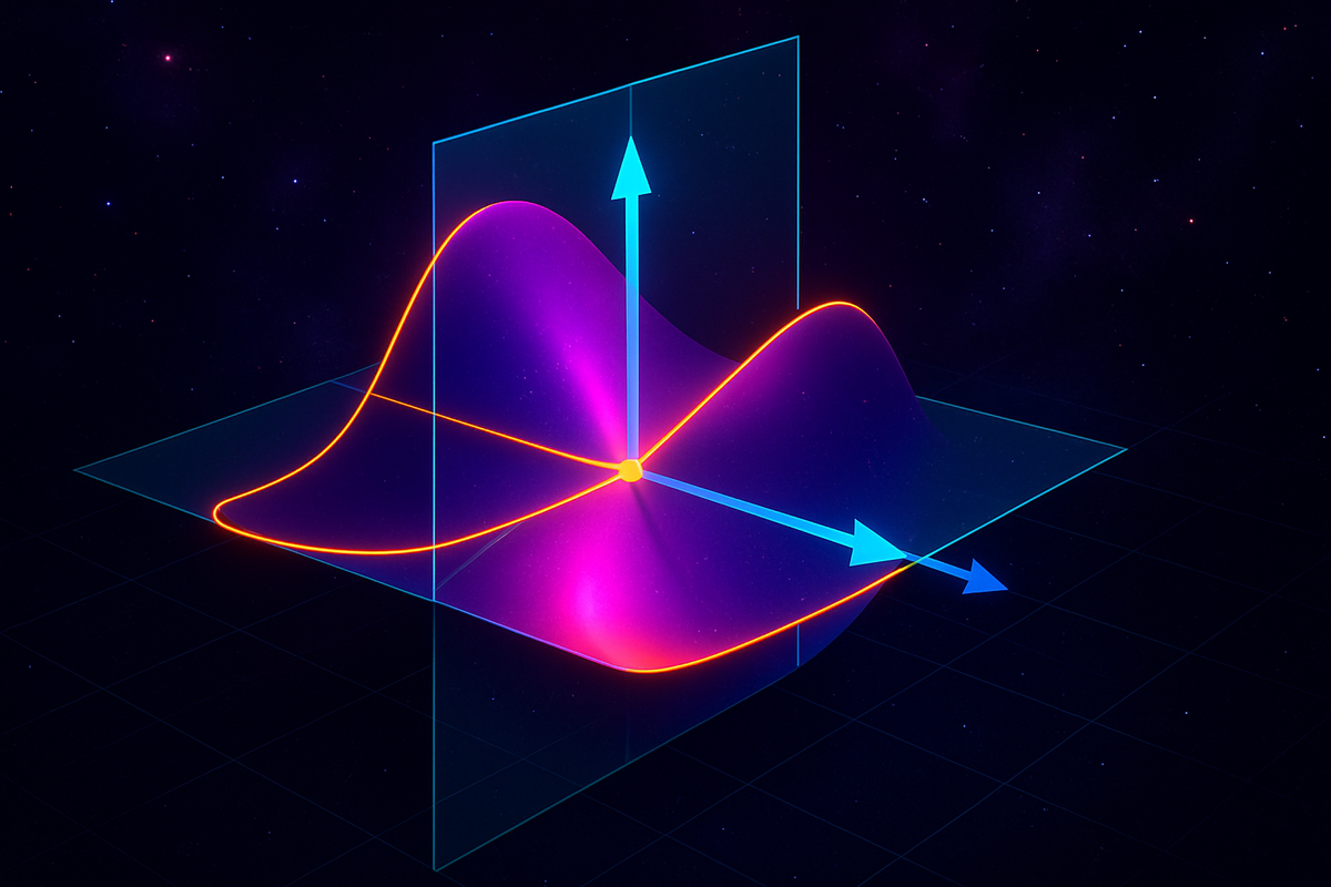
The Geometry: Slicing the Surface

Here's where partial derivatives get geometrically beautiful.

Consider z = f(x, y). This defines a surface in three-dimensional space. At every point (x, y) on the xy-plane, the function assigns a height z.

∂f/∂x is the slope of the surface in the x-direction. Imagine slicing the surface with a plane that's parallel to the xz-plane (constant y). You get a curve. The partial derivative ∂f/∂x is the slope of that curve.

∂f/∂y is the slope of the surface in the y-direction. Slice the surface with a plane parallel to the yz-plane (constant x). You get a different curve. The partial derivative ∂f/∂y is the slope of that curve.

In other words: partial derivatives measure how steeply the surface tilts when you move in directions parallel to the coordinate axes.

This is why the notation ∂f/∂x is powerful—it emphasizes that you're measuring a rate of change in a specific direction (the x-direction), not the overall "steepness" of the surface (that's what the gradient captures, but we'll get there).

Practical Interpretation: Ceteris Paribus

Economists will recognize partial derivatives as mathematical formalization of "ceteris paribus" analysis—holding all else equal.

Suppose f(x, y) represents profit, where x is advertising spend and y is production cost. Then:

∂f/∂x tells you how profit changes with increased advertising, assuming production cost stays fixed
∂f/∂y tells you how profit changes with increased production cost, assuming advertising spend stays fixed

This lets you reason about sensitivity to individual factors without the confounding effects of everything changing at once.

In physics, if T(x, y, t) is temperature at position (x, y) and time t, then:

∂T/∂x: temperature gradient in the eastward direction
∂T/∂y: temperature gradient in the northward direction
∂T/∂t: rate of temperature change over time at a fixed location

Each partial derivative isolates one dimension of variation.

Higher-Order Partial Derivatives

Just like you can take the derivative of a derivative in single-variable calculus (getting the second derivative), you can take partial derivatives of partial derivatives.

For f(x, y), there are four second-order partial derivatives:

∂²f/∂x² (or fₓₓ): Differentiate ∂f/∂x with respect to x again. This measures curvature in the x-direction.

∂²f/∂y² (or f_yy): Differentiate ∂f/∂y with respect to y again. This measures curvature in the y-direction.

∂²f/∂x∂y (or fₓᵧ): Differentiate ∂f/∂x with respect to y. This measures how the x-slope changes as you move in the y-direction.

∂²f/∂y∂x (or f_yx): Differentiate ∂f/∂y with respect to x. This measures how the y-slope changes as you move in the x-direction.

Here's something remarkable: for most functions you'll encounter (specifically, functions with continuous second partial derivatives), the mixed partials are equal:

∂²f/∂x∂y = ∂²f/∂y∂x

This is called Clairaut's theorem (or Schwarz's theorem, depending on your textbook). The order of differentiation doesn't matter.

Why does this matter? It's a constraint on how surfaces can bend. The fact that fₓᵧ = f_yx means you can't have a surface where the x-slope increases rapidly as you move in the y-direction but the y-slope barely changes as you move in the x-direction. The coupling is symmetric.

Example: Cobb-Douglas Production Function

Let's do a full example with economic flavor.

The Cobb-Douglas production function is Q(L, K) = AL^α K^β, where:

Q is output
L is labor input
K is capital input
A, α, β are constants (usually with α + β = 1 for constant returns to scale)

Let's take α = 0.6, β = 0.4, A = 10, so Q(L, K) = 10L^0.6 K^0.4.

Partial derivative with respect to L:

∂Q/∂L = 10 · 0.6 · L^(-0.4) · K^0.4 = 6L^(-0.4)K^0.4 = 6(K/L)^0.4

This is the marginal product of labor—how much additional output you get from one more unit of labor, holding capital fixed. Note that it decreases as L increases (diminishing returns).

Partial derivative with respect to K:

∂Q/∂K = 10 · L^0.6 · 0.4 · K^(-0.6) = 4L^0.6 K^(-0.6) = 4(L/K)^0.6

This is the marginal product of capital—how much additional output you get from one more unit of capital, holding labor fixed.

Second-order partial derivatives:

∂²Q/∂L² = 6 · (-0.4) · L^(-1.4) · K^0.4 = -2.4L^(-1.4)K^0.4

This is negative, confirming diminishing marginal returns to labor.

∂²Q/∂L∂K = 6 · 0.4 · L^(-0.4) · K^(-0.6) = 2.4L^(-0.4)K^(-0.6)

This is positive, meaning that increasing capital makes labor more productive (and vice versa, by symmetry of mixed partials). Labor and capital are complements, not substitutes.

All of this economic structure is encoded in the partial derivatives. The math isn't decorative—it's the formalization of how inputs interact to produce output.

When Partial Derivatives Don't Capture Everything

Here's a subtlety: knowing all the partial derivatives at a point tells you how the function changes if you move parallel to the coordinate axes. But what if you move diagonally? Or along a curve?

That's where directional derivatives come in (next article in the series). Partial derivatives are a special case of directional derivatives—they're the rates of change in the specific directions aligned with your chosen coordinate axes.

Also: partial derivatives are local information. They tell you about infinitesimal behavior near a point. They don't tell you about global structure—whether the function has a global maximum, whether it's bounded, whether it's continuous far from the point you're examining.

But within their domain—analyzing local sensitivity to individual variables—partial derivatives are indispensable.

The Notation Zoo: Different Ways to Write the Same Thing

Because partial derivatives are so central to multivariable calculus, there are many competing notations:

Leibniz notation: ∂f/∂x
Subscript notation: fₓ or f_x
Operator notation: ∂ₓf
Prime notation (less common for partials): f'ₓ

In physics, you'll often see subscripts indicating what's held constant:

(∂U/∂V)_T means: partial derivative of U with respect to V, holding T constant

In thermodynamics, this distinction matters because energy functions have many variables, and which ones you hold constant changes the physical meaning of the derivative.

For this series, we'll mostly stick with ∂f/∂x notation for clarity, occasionally using subscripts fₓ when it reduces clutter.

The Conceptual Core: Decomposition

The deeper idea behind partial derivatives is decomposition: a multivariable function's behavior can be understood by examining how it responds to changes in each variable independently.

This is reductionist thinking mathematized. You can't fully predict f(x, y, z) from knowing only ∂f/∂x, ∂f/∂y, and ∂f/∂z (you need mixed partials to capture interactions), but the partial derivatives are the first-order building blocks.

In linear algebra terms: the partial derivatives form the components of the gradient vector (which we'll explore next). The gradient is the proper multivariable generalization of the derivative, but it's built from partial derivatives as components.

In differential geometry terms: partial derivatives define the tangent plane to a surface at a point. The plane approximates the surface locally, just like a tangent line approximates a curve in single-variable calculus.

In optimization terms: critical points (where the function has maxima, minima, or saddle points) occur where all first-order partial derivatives are zero. Setting ∂f/∂x = 0, ∂f/∂y = 0 simultaneously gives you candidate locations for extrema.

Partial derivatives are the atoms from which the rest of multivariable calculus is built.

Computing Partial Derivatives: A Systematic Approach

When faced with a function f(x, y, z, ...), here's the systematic procedure:

Identify the variable you're differentiating with respect to. Call it x.
Treat all other variables as constants. They're just multiplicative factors that get carried along.
Apply standard differentiation rules (power rule, product rule, chain rule, etc.) to the terms involving x.
Simplify the result.

This works for polynomials, exponentials, trig functions, logarithms—everything. The only wrinkle is the chain rule when you have compositions, which we'll address in the multivariable chain rule article.

Example with exponentials: f(x, y) = e^(xy) + x² sin(y)

∂f/∂x = y·e^(xy) + 2x sin(y)

For e^(xy), chain rule: derivative of e^(xy) with respect to x is e^(xy) times derivative of xy with respect to x, which is y
For x² sin(y), sin(y) is constant, so just differentiate x² to get 2x

∂f/∂y = x·e^(xy) + x² cos(y)

For e^(xy), derivative with respect to y is e^(xy) times derivative of xy with respect to y, which is x
For x² sin(y), x² is constant, differentiate sin(y) to get cos(y)

The mechanics are straightforward once you internalize "other variables are constants."

Why This Matters

Partial derivatives are the foundation of:

Gradient descent: In machine learning, you optimize a loss function by computing its gradient (vector of partial derivatives) and stepping in the direction that decreases the loss fastest.

Thermodynamics: Equations of state relate pressure, volume, and temperature. Partial derivatives capture how these quantities respond to changes in the others, leading to Maxwell relations.

Elasticity in economics: Price elasticity of demand is essentially a partial derivative: how quantity demanded changes with price, holding other factors constant.

Sensitivity analysis: In any model with multiple parameters, partial derivatives tell you which parameters the output is most sensitive to—where small errors in estimation will have large effects.

Differential equations: Partial differential equations (like the heat equation, wave equation, Schrödinger equation) involve partial derivatives with respect to both space and time. They're the language of continuous physics.

You can't do modern quantitative analysis without fluency in partial derivatives. They're how you think about multidimensional sensitivity, how you optimize complex systems, how you model dynamics in space and time.

The Path Forward

Partial derivatives give you directional information: slopes along the x-axis, y-axis, z-axis, etc.

But surfaces don't just slope along coordinate axes. They slope in every direction. To capture the full richness of multidimensional change, you need to package partial derivatives into a vector—the gradient.

That's next. The gradient is where partial derivatives stop being separate numbers and start being components of a geometric object that points in the direction of steepest ascent.

Once you have gradients, you can talk about directional derivatives (slopes in arbitrary directions), optimization (finding where the gradient is zero), and the multivariable chain rule (how changes propagate through networks of dependent variables).

Partial derivatives are the alphabet. The gradient is where you start forming words. Let's keep building.

Part 2 of the Multivariable Calculus series.

Previous: What Is Multivariable Calculus? When Functions Have Multiple Inputs Next: The Gradient: All Partial Derivatives in One Vector