Basic Probability Rules: And Or and Not

Basic Probability Rules: And Or and Not | Ideasthesia

Three axioms. That's all.

From three simple statements—probabilities are non-negative, certainty has probability 1, mutually exclusive events add—everything else follows. Conditional probability, independence, Bayes' theorem, the entire machinery of statistics.

This article covers the working rules derived from those axioms. Master these, and you can calculate probabilities for any situation.

The Complement Rule

The probability of something not happening is 1 minus the probability it happens:

P(not A) = 1 - P(A)

This seems trivial. It isn't. "Not" calculations are often easier than direct ones.

Example: What's the probability of getting at least one head in five coin flips?

Direct calculation: Count outcomes with 1 head, 2 heads, 3, 4, 5. That's messy.

Complement: What's the probability of no heads? P(all tails) = (1/2)⁵ = 1/32

So: P(at least one head) = 1 - 1/32 = 31/32 ≈ 0.97

The complement trick turns hard problems easy.

The Addition Rule

For any two events A and B:

P(A or B) = P(A) + P(B) - P(A and B)

Why subtract the intersection? Because when you add P(A) and P(B), outcomes in both A and B get counted twice.

Example: Drawing a card. What's P(heart or face card)?

P(heart) = 13/52 P(face card) = 12/52 (3 per suit × 4 suits) P(heart AND face card) = 3/52 (J, Q, K of hearts)

P(heart or face card) = 13/52 + 12/52 - 3/52 = 22/52 ≈ 0.42

Special case—mutually exclusive events:

If A and B can't both happen, P(A and B) = 0, so:

P(A or B) = P(A) + P(B)

Rolling a 2 or 5 on a die: P(2 or 5) = 1/6 + 1/6 = 2/6 = 1/3

The Multiplication Rule

For any two events:

P(A and B) = P(A) × P(B | A)

The probability of both happening equals the probability of the first times the probability of the second given the first occurred.

Example: Drawing two cards without replacement. What's P(both aces)?

P(first ace) = 4/52 P(second ace | first was ace) = 3/51 (three aces left in 51 remaining cards)

P(both aces) = 4/52 × 3/51 = 12/2652 ≈ 0.0045

Independence

Two events are independent if knowing one occurred doesn't change the probability of the other:

P(A | B) = P(A)

Equivalently: P(A and B) = P(A) × P(B)

Examples of independent events:

Two coin flips
Two dice rolls
Separate random samples

Examples of dependent events:

Drawing cards without replacement (what's left affects probabilities)
Weather on consecutive days (today's weather affects tomorrow's)
Heights of family members (genetic correlation)

The multiplication rule for independent events:

P(A and B and C and ...) = P(A) × P(B) × P(C) × ...

Example: Probability of flipping heads five times in a row:

(1/2)⁵ = 1/32 ≈ 0.03

The General Multiplication Rule

For any sequence of events:

P(A₁ and A₂ and A₃ and ...) = P(A₁) × P(A₂|A₁) × P(A₃|A₁ and A₂) × ...

Each factor conditions on all previous events.

Example: Probability of drawing A♠, K♠, Q♠ in sequence from a deck:

P(A♠) = 1/52 P(K♠ | drew A♠) = 1/51 P(Q♠ | drew A♠ and K♠) = 1/50

P(all three) = 1/52 × 1/51 × 1/50 = 1/132,600 ≈ 0.0000075

The Law of Total Probability

If events B₁, B₂, ..., Bₙ partition the sample space (exactly one must occur), then:

P(A) = P(A|B₁)P(B₁) + P(A|B₂)P(B₂) + ... + P(A|Bₙ)P(Bₙ)

This is powerful. It lets you calculate a probability by breaking it into cases.

Example: A company has two factories. Factory 1 produces 60% of products with 2% defect rate. Factory 2 produces 40% with 5% defect rate. What fraction of all products are defective?

P(defective) = P(defective | Factory 1)P(Factory 1) + P(defective | Factory 2)P(Factory 2) = 0.02 × 0.60 + 0.05 × 0.40 = 0.012 + 0.020 = 0.032 = 3.2%

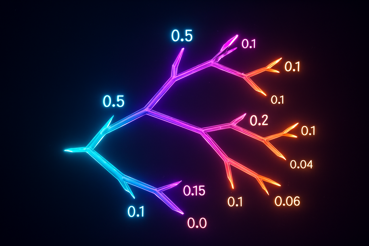
Tree Diagrams

For multi-step probability problems, tree diagrams visualize the calculation.

Each branch represents an outcome. Label branches with probabilities. Multiply along paths for "and." Add across paths for "or."

Example: You flip a coin. If heads, roll a die. If tails, draw a card.

        Heads (1/2) ──── Roll 1 (1/6) ──→ 1/12
                    ──── Roll 2 (1/6) ──→ 1/12
                    ──── Roll 3 (1/6) ──→ 1/12
                    ──── Roll 4 (1/6) ──→ 1/12
                    ──── Roll 5 (1/6) ──→ 1/12
                    ──── Roll 6 (1/6) ──→ 1/12

        Tails (1/2) ──── Heart (1/4) ──→ 1/8
                    ──── Diamond (1/4) ──→ 1/8
                    ──── Club (1/4) ──→ 1/8
                    ──── Spade (1/4) ──→ 1/8

P(roll 6) = P(heads) × P(6 | heads) = 1/2 × 1/6 = 1/12 P(heart drawn) = P(tails) × P(heart | tails) = 1/2 × 1/4 = 1/8

Counting Principles

When outcomes are equally likely, probability becomes counting:

P(A) = |A| / |Ω|

Counting techniques become probability techniques.

Multiplication principle: If task 1 has n₁ ways and task 2 has n₂ ways, together they have n₁ × n₂ ways.

Permutations: Arrangements where order matters. n! / (n-k)! ways to arrange k items from n

Combinations: Selections where order doesn't matter. C(n,k) = n! / (k!(n-k)!) = "n choose k"

Example: Probability of getting exactly 3 heads in 5 flips?

Number of ways to get 3 heads: C(5,3) = 10 Total outcomes: 2⁵ = 32 P(exactly 3 heads) = 10/32 = 5/16 ≈ 0.31

Common Patterns

At Least One: P(at least one A) = 1 - P(no A's)

None: P(no A's in n trials) = P(not A)ⁿ (if independent)

All: P(all A's in n trials) = P(A)ⁿ (if independent)

Exactly k: P(exactly k successes in n trials) = C(n,k) × pᵏ × (1-p)ⁿ⁻ᵏ

This last formula is the binomial distribution—it appears everywhere.

The Chain Rule

The general multiplication rule, restated:

P(A₁ ∩ A₂ ∩ ... ∩ Aₙ) = P(A₁) × P(A₂|A₁) × P(A₃|A₁,A₂) × ... × P(Aₙ|A₁,...,Aₙ₋₁)

This "chain rule" decomposes any joint probability into a product of conditionals. It's foundational for probabilistic models in machine learning.

Modern language models work this way. They generate text by computing P(next word | all previous words), multiplying conditional probabilities along the chain.

Examples That Trap Intuition

Example 1: The Monty Hall Problem

Three doors. One hides a car; two hide goats. You pick a door. The host (who knows what's behind each) opens a different door revealing a goat. Should you switch to the remaining door?

Answer: Yes. Switching wins 2/3 of the time.

Your initial pick has 1/3 chance of being right. The host's reveal doesn't change this—he always reveals a goat from the remaining doors. The remaining door gets the other 2/3.

Example 2: The False Positive Paradox

A drug test is 99% accurate (99% true positive rate, 99% true negative rate). If 1% of the population uses drugs, what's P(user | positive test)?

Using Bayes' theorem (covered next):

P(positive) = P(pos|user)P(user) + P(pos|non-user)P(non-user)
= 0.99 × 0.01 + 0.01 × 0.99 = 0.0198
P(user | positive) = P(pos|user)P(user) / P(positive)
= (0.99 × 0.01) / 0.0198 ≈ 0.50

A positive test only means 50% chance of actual use. Half of positives are false positives because non-users vastly outnumber users.

The Discipline of Probability

Working with probability requires discipline:

Always define the sample space. What are all possible outcomes? Getting this wrong ruins everything.

Check independence. Don't assume events are independent—verify it. Many errors come from assuming independence when events are correlated.

Use complements. "At least one" problems are almost always easier via "none."

Draw trees. For multi-step problems, tree diagrams prevent errors.

Condition explicitly. When probabilities depend on other information, write the condition. P(A) and P(A|B) are different quantities.

What's Next

These rules are tools. Conditional probability and Bayes' theorem are where the real power lies—the ability to update beliefs with evidence, reason backward from effects to causes, and make rational decisions under uncertainty.

That's next.

This is Part 2 of the Probability series. Next: "Conditional Probability: When Information Changes Everything."

Part 2 of the Probability series.

Previous: What Is Probability? Quantifying Uncertainty Next: Conditional Probability: When Information Changes the Odds