Recursion: Sequences Defined by Their Own Terms

A recursive sequence looks backward to go forward.

The Fibonacci sequence doesn't have a formula like aₙ = 2n + 1. It has a rule: each term is the sum of the previous two.

Fₙ = Fₙ₋₁ + Fₙ₋₂

This is recursion. The definition of term n involves earlier terms. The pattern contains itself.

Recursive definitions are everywhere: family trees, fractals, algorithms, population models. They're how mathematics describes things that grow from their own history.

The Structure of Recursion

A recursive definition has two parts:

1. Base case(s): Starting values that don't depend on previous terms
2. Recursive rule: How to compute new terms from previous ones

For Fibonacci:

• Base: F₁ = 1, F₂ = 1
• Rule: Fₙ = Fₙ₋₁ + Fₙ₋₂ for n ≥ 3

Without base cases, the recursion has nothing to start from. Without the rule, it has nothing to do.

The base cases are seeds. The rule is the growth law.

Linear Recurrences

The most tractable recursive sequences are linear recurrences:

aₙ = c₁aₙ₋₁ + c₂aₙ₋₂ + ... + cₖaₙ₋ₖ

Each term is a linear combination of the previous k terms.

First-order: aₙ = c₁aₙ₋₁

• Example: aₙ = 3aₙ₋₁ with a₁ = 2 gives 2, 6, 18, 54, ... (geometric)

Second-order: aₙ = c₁aₙ₋₁ + c₂aₙ₋₂

• Example: Fibonacci with c₁ = c₂ = 1

Higher-order: Tribonacci uses the previous three terms.

Linear recurrences have a beautiful theory: they can always be solved using characteristic equations.

Solving Linear Recurrences

For aₙ = c₁aₙ₋₁ + c₂aₙ₋₂, the characteristic equation is:

r² = c₁r + c₂, or r² - c₁r - c₂ = 0

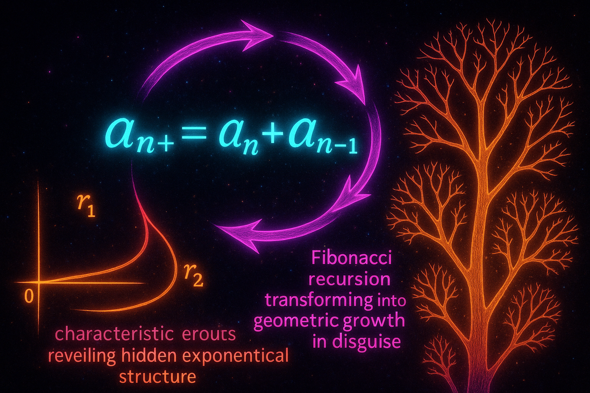
If this has roots r₁ and r₂ (distinct), the general solution is:

aₙ = Ar₁ⁿ + Br₂ⁿ

A and B are determined by the base cases.

Example: Fibonacci

Fₙ = Fₙ₋₁ + Fₙ₋₂. Characteristic equation: r² = r + 1.

Roots: r = (1 ± √5)/2. Call them φ ≈ 1.618 and ψ ≈ -0.618.

General solution: Fₙ = Aφⁿ + Bψⁿ.

Using F₁ = 1, F₂ = 1 to solve for A and B:

Fₙ = (φⁿ - ψⁿ)/√5

This is Binet's formula. A recursive sequence turns out to be a sum of exponentials.

When Roots Repeat

If the characteristic equation has a repeated root r, the solution changes:

aₙ = (A + Bn)rⁿ

The factor of n accounts for the repeated root.

Example: aₙ = 4aₙ₋₁ - 4aₙ₋₂ with a₁ = 1, a₂ = 4.

Characteristic equation: r² - 4r + 4 = (r-2)² = 0. Repeated root r = 2.

General solution: aₙ = (A + Bn)2ⁿ.

Using base cases: 1 = (A + B)2, 4 = (A + 2B)4.

Solving gives A = 0, B = 1/2, so aₙ = (n/2)2ⁿ = n·2ⁿ⁻¹.

Non-Homogeneous Recurrences

Some recurrences have extra terms:

aₙ = 2aₙ₋₁ + n

This is non-homogeneous (the n term doesn't fit the pattern).

Solution method:

1. Solve the homogeneous version (aₙ = 2aₙ₋₁) to get the general solution
2. Find a particular solution to the full equation
3. Add them

The particular solution often has the same form as the extra term. If the extra term is n, try aₙ = An + B.

Famous Recursive Sequences

Factorials: n! = n × (n-1)!, with 0! = 1.

Lucas numbers: Like Fibonacci but starting with 2, 1: Lₙ = Lₙ₋₁ + Lₙ₋₂.

Gives 2, 1, 3, 4, 7, 11, 18, ...

Tower of Hanoi: Tₙ = 2Tₙ₋₁ + 1 with T₁ = 1.

Gives 1, 3, 7, 15, 31, ... = 2ⁿ - 1.

Catalan numbers: Cₙ = ∑ᵢ₌₀ⁿ⁻¹ CᵢCₙ₋₁₋ᵢ

A more complex recursion that counts binary trees, valid parentheses, and dozens of combinatorial objects.

Recursion in Algorithms

Computer scientists love recursion because it turns complex problems into simple patterns.

Merge sort: To sort a list, split it in half, sort each half recursively, then merge.

T(n) = 2T(n/2) + O(n)

This recurrence gives T(n) = O(n log n).

Binary search: To find a value, check the middle, then recurse on the appropriate half.

T(n) = T(n/2) + O(1)

This gives T(n) = O(log n).

The Master Theorem provides formulas for recurrences of the form T(n) = aT(n/b) + f(n).

Recursion vs. Closed Form

A closed form expresses aₙ directly in terms of n:

Fibonacci: Fₙ = (φⁿ - ψⁿ)/√5 (closed form) Fibonacci: Fₙ = Fₙ₋₁ + Fₙ₋₂ (recursive)

Both define the same sequence. Closed forms are efficient for computing single terms. Recursive definitions reveal structure and are often easier to discover.

Not all recursive sequences have nice closed forms. The Catalan numbers have a closed form:

Cₙ = (2n)! / ((n+1)!n!)

But many sequences don't simplify so cleanly.

The Danger of Naive Recursion

Computing Fibonacci recursively without memory is disastrously slow:

fib(n) = fib(n-1) + fib(n-2)

To compute fib(50), this makes roughly 2⁵⁰ calls. That's over 10¹⁵ operations.

The problem: overlapping subproblems. fib(48) gets computed twice when computing fib(50). fib(47) gets computed four times. The redundancy explodes.

Solution: Memoization or dynamic programming

Store results as you compute them. Compute fib(1), fib(2), fib(3), ... in order. Each term takes O(1) time. Total: O(n).

Naive recursion can be exponential. Smart recursion is linear.

Mutual Recursion

Sometimes two sequences define each other:

aₙ = bₙ₋₁ + 1 bₙ = aₙ₋₁ × 2

Each sequence depends on the other. You can often combine them into a single sequence or solve them simultaneously.

Mutual recursion appears in grammar (sentences contain clauses, clauses contain phrases, phrases contain sentences) and in mathematical definitions (even and odd numbers can be defined mutually).

Why Recursion Matters

1. It captures self-reference. Many real patterns define themselves: trees have branches that are smaller trees.
2. It's natural for mathematics. Factorials, Fibonacci, binomial coefficients—many fundamental sequences are recursive.
3. It's the foundation of algorithms. Divide-and-conquer, dynamic programming, and backtracking all use recursive structure.
4. It connects to closed forms. Solving recurrences reveals that many recursive patterns are secretly exponential.
5. It's how computation works. Recursive functions are as powerful as any other model of computation (Church-Turing thesis).

The recursive sequence says: to understand where you're going, look at where you've been. The future is defined by the past.

Part 11 of the Sequences Series series.

Previous: Power Series: Polynomials That Go On Forever Next: Synthesis: Sequences and Series as the Language of Patterns