Spikes Not Floats: How Biological Neurons Actually Compute

Series: Neuromorphic Computing | Part: 2 of 9

If you've ever taken an intro AI course, you've been lied to about neurons. Not maliciously—the simplification was necessary. But the gap between artificial neural networks and biological neurons isn't just a matter of complexity. It's a fundamental difference in computational paradigm. One uses continuous activations flowing through weighted connections. The other uses discrete electrical spikes arriving at precise moments in time.

The difference matters because we're now building hardware that works like real brains. And to understand why neuromorphic chips will outperform GPUs for certain tasks by orders of magnitude, we need to understand what biological neurons actually do.

This isn't just neuroscience trivia. It's the foundation for a revolution in computation.

The Textbook Neuron Is a Cartoon

In deep learning, a neuron is embarrassingly simple: it receives weighted inputs, sums them, applies a nonlinear activation function, and outputs a number. That number might be interpreted as a firing rate, but it's really just a scalar—a single continuous value passed to the next layer.

This model traces back to McCulloch and Pitts (1943), who formalized neurons as logical threshold units. Rosenblatt's perceptron (1958) added learning. Backpropagation (1986) made it scalable. And suddenly we had a computational framework powerful enough to recognize faces, translate languages, and beat humans at Go.

But biological neurons don't work like this. At all.

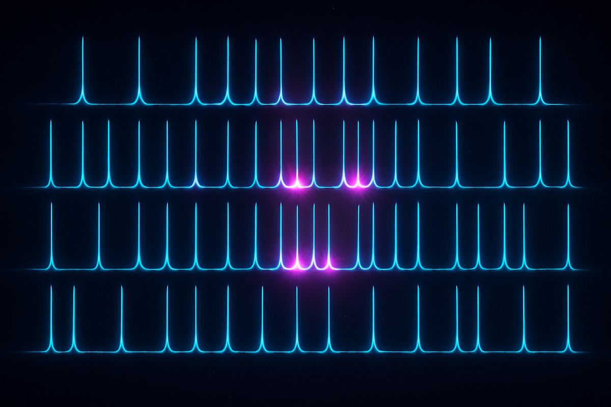
Real neurons communicate through action potentials—stereotyped electrical pulses, roughly 100 millivolts in amplitude and 1-2 milliseconds in duration. These spikes are all-or-nothing events. There's no gradation in spike amplitude. A neuron either fires or it doesn't.

The information isn't in the size of the spike. It's in the pattern of spikes across time.

This is spike-based computation, and it operates under entirely different principles than the weighted-sum-then-activate paradigm of artificial neural networks.

What a Spike Actually Is

To understand spiking computation, start with the biophysics. A neuron at rest maintains a membrane potential around -70 millivolts, pumped into place by ion channels that actively segregate sodium and potassium. When excitatory inputs push the membrane potential past a threshold (typically around -55 mV), voltage-gated sodium channels snap open. Sodium floods in. The membrane potential spikes to +40 mV.

Then, just as quickly, the sodium channels close and potassium channels open. Potassium flows out. The membrane potential plummets back below resting, briefly hyperpolarizing before the cell stabilizes. The whole event lasts 1-2 milliseconds.

This is the action potential. It propagates down the axon to synaptic terminals, where it triggers neurotransmitter release, which in turn causes post-synaptic potentials (PSPs) in downstream neurons. Those PSPs can be excitatory (pushing the membrane potential up) or inhibitory (pushing it down).

If enough excitatory PSPs arrive in a short window—say, 10-20 milliseconds—their effects sum, and the post-synaptic neuron crosses threshold and fires its own spike.

So far, this sounds like it could be approximated by a weighted sum and threshold. And to first order, that's not entirely wrong. But here's where the analogy breaks down: timing matters.

Spike Timing Is Information

In artificial neural networks, timing is irrelevant. A neuron's activation is computed once per forward pass. It doesn't matter if input A arrived before input B or simultaneously—they're just summed.

In biology, the order and precise timing of spikes encodes information that the rate alone cannot capture.

Consider temporal coding. Neurons in the auditory system of barn owls can distinguish time differences as small as 10 microseconds between spikes arriving at the two ears. This is how owls localize sound in the dark—by detecting interaural time differences at microsecond precision. No rate code could achieve this. The information is in the spike timing itself.

Or consider spike-timing-dependent plasticity (STDP), discovered by Markram, Lübke, Frotscher, and Sakmann (1997). If a pre-synaptic neuron fires just before a post-synaptic neuron (within ~20 milliseconds), the synapse strengthens. If the pre-synaptic spike arrives just after, the synapse weakens. This is a causal learning rule: the synapse learns to predict which inputs cause the neuron to fire.

No Hebbian "neurons that fire together wire together" here—the order matters. Timing is the learning signal.

Then there's synchrony. Groups of neurons firing in tight temporal coordination (~1-5 ms windows) can have dramatically different effects than the same number of spikes arriving asynchronously. Synchronized spikes create sharp, high-amplitude post-synaptic potentials. Asynchronous spikes create a noisy, diffuse signal. The brain uses synchrony to bind features (the "binding problem" in neuroscience), to route information (communication-through-coherence hypothesis), and to coordinate activity across distant regions.

None of this is captured by rate codes. The spike train isn't just a noisy version of a continuous signal. It's a discrete event sequence where timing and pattern carry meaning.

Why Biology Uses Spikes

If continuous signals are mathematically convenient (and they are—calculus works beautifully on smooth functions), why does biology bother with discrete, sparse spikes?

The answer is energy efficiency.

Neurons spend most of their energy budget on the sodium-potassium pump, maintaining the ionic gradients that enable action potentials. But once those gradients are established, generating a spike is relatively cheap—because spikes are passive once initiated. The voltage-gated channels open in a cascade; no additional ATP required for the spike itself.

Compare this to continuously transmitting an analog signal, which would require constant energy expenditure to maintain a graded voltage. In a brain with 86 billion neurons, each making thousands of connections, the energetic cost of continuous signaling would be prohibitive.

Spikes are biology's solution to the communication bandwidth problem in a system constrained by energy. By encoding information in the timing and pattern of sparse, discrete events, neurons transmit rich information at minimal metabolic cost.

This is why a human brain running on ~20 watts can outperform a GPU cluster drawing 100,000 watts for many tasks. The computational substrate is fundamentally different.

Spike Codes in the Wild

So what do real spike patterns look like? Here are a few canonical examples:

Rate coding is the simplest: information is in the average firing rate over a time window (typically 50-200 ms). A neuron firing at 10 Hz might encode a dim light; 50 Hz, a bright light. This is the most direct analogue to artificial neural networks, and it's the most commonly assumed code in systems neuroscience. It's also probably not the whole story.

Temporal coding encodes information in precise spike times. In the locust olfactory system, individual neurons respond to odors with stereotyped, millisecond-precise spike patterns (Laurent, 2002). The pattern, not just the rate, identifies the odor. Similarly, hippocampal place cells don't just fire when an animal enters a location—they fire at specific phases of the theta oscillation (~8 Hz), encoding position within the theta cycle (phase precession).

Population coding distributes information across many neurons. A single neuron might be noisy, but a population of neurons with overlapping tuning curves can encode information with high precision. This is how motor cortex controls movement: no single neuron encodes "move arm left"—populations of neurons collectively specify movement direction and velocity.

Burst coding uses clusters of spikes in rapid succession (interspike intervals of 2-10 ms) to signal salience or novelty. Bursts are more reliable in driving post-synaptic spikes than single spikes, making them useful for urgent or high-priority signals.

Synchrony coding uses coordinated firing across neurons to bind features or gate information flow. Gamma oscillations (~40 Hz) in visual cortex are thought to synchronize neurons representing different features of the same object, solving the binding problem.

These aren't mutually exclusive. Real neurons likely use multiple codes depending on context. But all of them rely on the event-based nature of spikes.

Spikes as Discrete Events, Not Continuous Signals

Here's the conceptual leap: biological neurons aren't computing continuous functions. They're processing discrete event streams.

Each incoming spike is an event. It arrives at a specific time, at a specific synapse, with a specific weight (efficacy). The neuron integrates these events—not by summing continuous values, but by accumulating transient perturbations to its membrane potential. If enough events arrive within the integration window (typically 10-50 ms), the neuron crosses threshold and emits its own event.

This is fundamentally asynchronous computation. Neurons don't wait for a clock signal. They don't process inputs in lockstep. They respond to events as they arrive, in continuous time.

Contrast this with deep learning, where computation is synchronous: all neurons in a layer compute their activations simultaneously, wait for all activations to be computed, then pass them to the next layer. This requires global coordination—a clock, or at least a scheduler.

Biological brains don't have global clocks. They don't need them. Event-based computation is naturally asynchronous. And this is one reason why neuromorphic hardware, which mimics this event-driven paradigm, can achieve dramatic efficiency gains over synchronous GPUs.

The Integration Window and Temporal Credit Assignment

One underappreciated consequence of spike-based computation is the temporal credit assignment problem. When a neuron fires, which of its recent inputs deserve credit?

In backpropagation through time (BPTT), used in recurrent neural networks, gradients are computed explicitly across time steps. This is computationally expensive and requires storing activations across many time steps.

In biology, credit assignment happens locally through STDP and related plasticity rules. Pre-synaptic spikes that arrived just before the post-synaptic spike get strengthened. Those that arrived just after get weakened. No global backpropagation required.

This local, temporally asymmetric learning rule is biologically plausible. It's also computationally efficient—neurons don't need to know the global error signal or store long sequences of past activations. They just need to remember recent spike times and adjust synapses accordingly.

But STDP alone isn't enough to train deep networks. Researchers are still figuring out how to combine STDP-like local rules with some form of error feedback to achieve the performance of backpropagation. This is an active frontier in neuromorphic computing research.

Why This Matters for Neuromorphic Hardware

Now we can see why neuromorphic hardware—chips designed to implement spiking neurons—has the potential to revolutionize computation.

First, energy efficiency. GPUs burn power because they compute continuously, updating billions of floating-point activations in lockstep. Neuromorphic chips compute only when spikes arrive. Most of the time, most neurons are silent. This sparse, event-driven computation saves orders of magnitude in power.

Second, latency. Synchronous systems require waiting for the slowest operation before proceeding to the next layer. Neuromorphic systems are asynchronous—information flows as soon as spikes are emitted, without waiting for a clock. This enables real-time sensorimotor loops with sub-millisecond latency.

Third, scalability. Spiking neural networks scale naturally to millions of neurons because there's no global synchronization bottleneck. Each neuron operates independently, responding to events as they arrive. This is how brains scale to billions of neurons without collapsing under coordination overhead.

Fourth, temporal computation. Many real-world tasks—speech recognition, motor control, navigation—are inherently temporal. Spikes are native representations of events in time. Neuromorphic hardware handles temporal patterns naturally, without the awkward workarounds (recurrent layers, attention over time steps) required in deep learning.

None of this means neuromorphic chips will replace GPUs for all tasks. For training large language models on static datasets, GPUs are unbeatable. But for edge AI, robotics, sensor fusion, and any task requiring real-time temporal processing with tight power budgets, neuromorphic hardware is the future.

And that future depends on understanding what biological neurons actually do: process discrete spikes in continuous time, with timing and pattern carrying the signal.

Spikes Are the Computation

The textbook neuron is a useful fiction. It enables backpropagation, gradient descent, and the entire edifice of modern deep learning. But it's not how brains compute.

Brains use spikes—discrete, sparse, precisely timed events. The timing encodes information. The sparsity saves energy. The asynchrony enables scalability. And the event-driven paradigm mirrors the structure of the physical world, where information arrives as events, not as smoothly varying signals.

If we want to build hardware that thinks like brains—not just mimics their architecture but captures their computational principles—we need to embrace spikes. Not as a discretized approximation of a continuous signal, but as the fundamental unit of neural computation.

Spikes, not floats. Events, not activations. Timing, not just magnitude.

This is the computational language of biology. And it's the key to the neuromorphic revolution.

Series: Neuromorphic Computing | Part: 2 of 9

Previous: The Chips That Think Like Brains: Inside the Neuromorphic Computing Revolution

Next: Intel Loihi and the Race for Brain-Like Silicon

Further Reading

• Gerstner, W., Kistler, W. M., Naud, R., & Paninski, L. (2014). Neuronal Dynamics: From Single Neurons to Networks and Models of Cognition. Cambridge University Press.
• Izhikevich, E. M. (2007). "Dynamical Systems in Neuroscience: The Geometry of Excitability and Bursting." MIT Press.
• Markram, H., Lübke, J., Frotscher, M., & Sakmann, B. (1997). "Regulation of synaptic efficacy by coincidence of postsynaptic APs and EPSPs." Science, 275(5297), 213-215.
• Laurent, G. (2002). "Olfactory network dynamics and the coding of multidimensional signals." Nature Reviews Neuroscience, 3(11), 884-895.
• Maass, W. (1997). "Networks of spiking neurons: The third generation of neural network models." Neural Networks, 10(9), 1659-1671.
• Thorpe, S., Delorme, A., & Van Rullen, R. (2001). "Spike-based strategies for rapid processing." Neural Networks, 14(6-7), 715-725.