Triple Integrals: Integrating Through Volumes

Triple Integrals: Integrating Through Volumes | Ideasthesia

Double integrals sum over regions in two dimensions. Triple integrals? They sum over volumes in three dimensions.

This is the full spatial version of integration: accumulating quantities throughout a solid, computing total mass when density varies in all three directions, finding moments of inertia for 3D objects, calculating gravitational or electric fields generated by continuous charge distributions.

Triple integrals are conceptually identical to double integrals—you're just adding one more dimension. But that extra dimension creates geometric complexity: regions become 3D solids, limits become surfaces, visualization requires slicing through volumes.

Mastering triple integrals means internalizing how to describe three-dimensional regions mathematically and how to integrate over them methodically.

The Setup: Integrating Over a Volume

A triple integral over a volume V in 3D space is written:

∭_V f(x, y, z) dV

where dV is an infinitesimal volume element.

If f represents density ρ(x, y, z), the integral gives total mass. If f is temperature T(x, y, z), the integral gives total thermal energy (when multiplied by heat capacity). If f = 1, the integral gives the volume of V.

Geometrically, you're partitioning the volume V into tiny boxes of volume ΔV, evaluating f at a point in each box, summing f(x, y, z) ΔV over all boxes, then taking the limit as ΔV → 0.

Computing Triple Integrals: Three Nested Integrals

Just as double integrals reduce to two nested single-variable integrals, triple integrals reduce to three:

∭V f(x, y, z) dV = ∫a^b ∫{g₁(x)}^{g₂(x)} ∫{h₁(x,y)}^{h₂(x,y)} f(x, y, z) dz dy dx

The order can vary: dz dy dx, dy dz dx, dx dz dy, etc. There are six possible orders, and choosing the right one can simplify computation dramatically.

How to set limits:

The outermost integral has constant limits (the range of the first variable).
The middle integral's limits can depend on the first variable.
The innermost integral's limits can depend on both the first and second variables.

You're slicing the volume three times: first along one axis to get a range, then slicing each slice to get a region, then slicing each region to get an interval.

Example 1: Rectangular box

Let V be the box [0, 2] × [0, 3] × [0, 4] (0 ≤ x ≤ 2, 0 ≤ y ≤ 3, 0 ≤ z ≤ 4).

Compute ∭_V (x + y + z) dV.

∭_V (x + y + z) dV = ∫₀² ∫₀³ ∫₀⁴ (x + y + z) dz dy dx

Innermost integral (integrate with respect to z):

∫₀⁴ (x + y + z) dz = [(x + y)z + z²/2]₀⁴ = 4(x + y) + 8

Middle integral (integrate with respect to y):

∫₀³ [4(x + y) + 8] dy = [4xy + 2y² + 8y]₀³ = 12x + 18 + 24 = 12x + 42

Outermost integral (integrate with respect to x):

∫₀² (12x + 42) dx = [6x² + 42x]₀² = 24 + 84 = 108

So ∭_V (x + y + z) dV = 108.

For a rectangular box, all six orders of integration give the same limits and the same answer (though intermediate steps differ).

Non-Rectangular Regions: Describing 3D Solids

For non-box regions, setting limits requires understanding the geometry.

Type 1 (z-simple): For each (x, y) in a region R in the xy-plane, z ranges from z₁(x, y) to z₂(x, y).

∭_V f(x, y, z) dV = ∬R ∫{z₁(x,y)}^{z₂(x,y)} f(x, y, z) dz dA

where dA = dy dx or dx dy depending on how you handle the double integral over R.

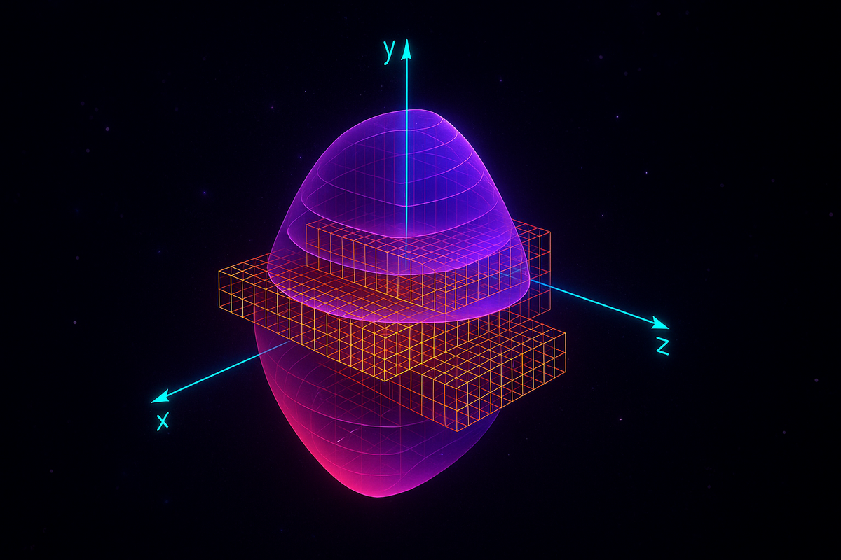
Example: The solid bounded by the paraboloid z = x² + y² (below) and the plane z = 4 (above).

For each (x, y) in the disk x² + y² ≤ 4 (the projection of the region onto the xy-plane), z ranges from x² + y² to 4.

If we use Cartesian coordinates for the disk (not optimal, but possible):

∭V f(x, y, z) dV = ∫{-2}² ∫{-√(4-x²)}^{√(4-x²)} ∫{x²+y²}⁴ f(x, y, z) dz dy dx

The innermost integral is over z from the paraboloid to the plane. The middle integral is over y from the bottom to top of the disk at that x. The outermost integral is over x across the disk.

This is correct but messy. Cylindrical coordinates (which we'll cover in the Jacobian article) make this trivial.

Type 2 (y-simple) and Type 3 (x-simple): Similarly, you can describe regions where x or y varies between surfaces, with projections onto other coordinate planes.

The key is always: identify the projection of the volume onto a coordinate plane, then determine how the third variable ranges over that projection.

Volume of a Region

Setting f = 1 gives the volume of V:

Volume(V) = ∭_V 1 dV

Example: Find the volume of the tetrahedron with vertices (0, 0, 0), (1, 0, 0), (0, 1, 0), (0, 0, 1).

This tetrahedron is bounded by the coordinate planes (x ≥ 0, y ≥ 0, z ≥ 0) and the plane x + y + z = 1.

For a given x in [0, 1], y ranges from 0 to 1 - x (projecting onto the xy-plane). For a given (x, y), z ranges from 0 to 1 - x - y (up to the plane).

Volume = ∫₀¹ ∫₀^{1-x} ∫₀^{1-x-y} 1 dz dy dx

Innermost integral:

∫₀^{1-x-y} 1 dz = 1 - x - y

Middle integral:

∫₀^{1-x} (1 - x - y) dy = [(1 - x)y - y²/2]₀^{1-x} = (1 - x)² - (1 - x)²/2 = (1 - x)²/2

Outermost integral:

∫₀¹ (1 - x)²/2 dx = (1/2)[-(1 - x)³/3]₀¹ = (1/2)(1/3) = 1/6

The volume of the tetrahedron is 1/6.

This is a standard result: the volume of a tetrahedron with one vertex at the origin and three edges along the coordinate axes of lengths a, b, c is abc/6. Here a = b = c = 1, so volume = 1/6.

Mass and Density in 3D

If ρ(x, y, z) is the density (mass per unit volume) at point (x, y, z), then the total mass of the solid V is:

M = ∭_V ρ(x, y, z) dV

Example: A solid sphere of radius R has density ρ(x, y, z) = k(x² + y² + z²) (density increases with distance from the center).

The mass is:

M = ∭_{x²+y²+z²≤R²} k(x² + y² + z²) dV

In Cartesian coordinates, this is a nightmare to set up (the sphere's limits involve nested square roots).

In spherical coordinates (ρ, θ, φ), where x² + y² + z² = ρ², the region is simply 0 ≤ ρ ≤ R, 0 ≤ θ ≤ 2π, 0 ≤ φ ≤ π, and the integral becomes:

M = ∫₀^{2π} ∫₀^π ∫₀^R k ρ² · ρ² sin φ dρ dφ dθ

(The ρ² sin φ factor is the Jacobian for spherical coordinates.)

This is much simpler. The moral: choose coordinates that match the symmetry of the problem.

We'll explore this in detail in the Jacobian article.

Center of Mass in 3D

The center of mass (x̄, ȳ, z̄) of a solid V with density ρ(x, y, z) is:

x̄ = (1/M) ∭_V x ρ(x, y, z) dV

ȳ = (1/M) ∭_V y ρ(x, y, z) dV

z̄ = (1/M) ∭_V z ρ(x, y, z) dV

where M = ∭_V ρ(x, y, z) dV is the total mass.

These are weighted averages of the coordinates, weighted by density.

Example: A solid hemisphere of radius R (upper half of a sphere, z ≥ 0) with uniform density ρ = 1.

By symmetry, x̄ = ȳ = 0 (the center of mass lies on the z-axis).

Find z̄.

The volume (which equals mass since ρ = 1) of a hemisphere is (2/3)πR³.

z̄ = (1/M) ∭_V z dV

In spherical coordinates, z = ρ cos φ, and the hemisphere is 0 ≤ ρ ≤ R, 0 ≤ θ ≤ 2π, 0 ≤ φ ≤ π/2.

The volume element in spherical coordinates is dV = ρ² sin φ dρ dφ dθ.

∭_V z dV = ∫₀^{2π} ∫₀^{π/2} ∫₀^R (ρ cos φ) ρ² sin φ dρ dφ dθ

= ∫₀^{2π} dθ ∫₀^{π/2} cos φ sin φ dφ ∫₀^R ρ³ dρ

= 2π · [sin²φ/2]₀^{π/2} · [ρ⁴/4]₀^R

= 2π · (1/2) · (R⁴/4) = πR⁴/4

So z̄ = (πR⁴/4) / [(2/3)πR³] = (πR⁴/4) · (3/(2πR³)) = 3R/8.

The center of mass of a uniform hemisphere is at height 3R/8 above the base—closer to the base than the top, as expected for a hemisphere.

Moments of Inertia

The moment of inertia of a solid about an axis measures its resistance to rotation about that axis.

For rotation about the z-axis, the moment of inertia is:

I_z = ∭_V (x² + y²) ρ(x, y, z) dV

where x² + y² is the square of the distance from the z-axis.

For rotation about other axes, you use the appropriate distance formula.

Moments of inertia are crucial in physics and engineering for analyzing rotational dynamics.

Choosing the Order of Integration

With three variables, there are six possible orders: dz dy dx, dz dx dy, dy dz dx, dy dx dz, dx dz dy, dx dy dz.

The choice depends on:

The geometry of the region (which surfaces bound it)
Which order makes the limits simplest
Which order makes the integrand easiest to integrate

General strategy:

Sketch the region (or at least understand its geometry)
Identify which surfaces bound it (spheres, planes, paraboloids, etc.)
Choose coordinates (Cartesian, cylindrical, spherical) that match the symmetry
Choose the integration order that gives the simplest limits

For regions with circular or cylindrical symmetry, cylindrical coordinates (r, θ, z) are often best. For regions with spherical symmetry, spherical coordinates (ρ, θ, φ) are often best. For rectangular boxes or regions bounded by planes, Cartesian coordinates work fine.

Example: Sphere Using Different Orders

Find the volume of a sphere of radius R.

Using z-simple in Cartesian coordinates:

The sphere is x² + y² + z² ≤ R².

Project onto the xy-plane: the disk x² + y² ≤ R².

For each (x, y) in the disk, z ranges from -√(R² - x² - y²) to √(R² - x² - y²).

Volume = ∬{x²+y²≤R²} ∫{-√(R²-x²-y²)}^{√(R²-x²-y²)} 1 dz dA

= ∬_{x²+y²≤R²} 2√(R² - x² - y²) dA

Now integrate over the disk. In Cartesian coordinates:

= ∫{-R}^R ∫{-√(R²-x²)}^{√(R²-x²)} 2√(R² - x² - y²) dy dx

This is doable but involves elliptic integrals or clever trig substitutions.

Using spherical coordinates:

In spherical coordinates, the sphere is simply 0 ≤ ρ ≤ R, 0 ≤ θ ≤ 2π, 0 ≤ φ ≤ π.

The volume element is dV = ρ² sin φ dρ dφ dθ.

Volume = ∫₀^{2π} ∫₀^π ∫₀^R ρ² sin φ dρ dφ dθ

= ∫₀^{2π} dθ ∫₀^π sin φ dφ ∫₀^R ρ² dρ

= 2π · [-cos φ]₀^π · [ρ³/3]₀^R

= 2π · 2 · (R³/3) = (4/3)πR³

The standard formula for the volume of a sphere, obtained with minimal effort.

The lesson: matching coordinates to symmetry transforms hard integrals into easy ones.

Applications of Triple Integrals

Physics:

Gravitational potential: ∭_V G ρ(x, y, z) / r dV where r is distance to a point
Electromagnetic fields: ∭_V ρ(x, y, z) r/r³ dV for field due to charge distribution
Fluid dynamics: ∭_V v(x, y, z) ρ(x, y, z) dV for total momentum

Engineering:

Moments of inertia for 3D bodies
Center of mass for irregular objects
Total heat energy in a solid with varying temperature

Probability:

If p(x, y, z) is a 3D probability density, ∭_V p(x, y, z) dV is the probability that (X, Y, Z) lies in V

Geometry:

Volume of solids bounded by surfaces
Surface area via triple integrals (using divergence theorem)

Every application boils down to: "sum this quantity throughout this volume."

Fubini's Theorem in Three Dimensions

As with double integrals, the order of integration doesn't affect the result (assuming f is continuous or integrable):

∫∫∫ f(x, y, z) dz dy dx = ∫∫∫ f(x, y, z) dy dz dx = ... (any of the six orders)

You can choose whichever order makes the computation tractable.

Visualization: Slicing the Volume

One way to visualize a triple integral: think of slicing the volume into thin slabs.

For ∫∫∫ f(x, y, z) dz dy dx:

First, fix x and y. Integrate over z to get a value (collapsing the z-dimension into a number).
This gives you a function of x and y: ∫ f(x, y, z) dz = g(x, y).
Now you have a double integral: ∬ g(x, y) dy dx, which you compute as before.

Alternatively, for ∫∫∫ f(x, y, z) dz dy dx:

First, integrate over z for each fixed (x, y), getting g(x, y).
Then integrate g over y for each fixed x, getting h(x).
Finally, integrate h over x to get the final number.

Each integration collapses one dimension, reducing the problem step by step.

When Triple Integrals Are Hard

Triple integrals are hard when:

The region's boundary is geometrically complex (integrals of surfaces that aren't simple formulas)
The integrand f has no elementary antiderivative
The chosen coordinate system doesn't match the problem's symmetry

Solutions:

Change coordinates (cylindrical, spherical, or even custom coordinates)
Use symmetry to simplify (if the region or integrand has symmetry, exploit it)
Approximate numerically (Monte Carlo integration, numerical quadrature)

For most textbook problems, choosing the right coordinates and integration order makes the integral tractable.

The Conceptual Core: Accumulation in 3D

Single integrals sum along a line (1D). Double integrals sum over a region (2D). Triple integrals sum throughout a volume (3D).

The pattern extends: you could define quadruple integrals over 4D regions, and so on. The mechanics are the same—nested integrals, one per dimension.

But physically, we live in 3D space (plus time), so triple integrals are as far as spatial accumulation goes for most applications.

The conceptual move is always the same: partition the domain into infinitesimal pieces, sum the quantity over those pieces, take the limit.

Calculus in multiple dimensions is just organized summation with limits.

What's Next

Triple integrals complete the basic integration toolkit for multivariable calculus.

Next, we tackle the Jacobian and change of variables: how to transform integrals from one coordinate system to another (Cartesian to polar, cylindrical, spherical, or arbitrary transformations).

This is where the r dr dθ in polar coordinates and the ρ² sin φ dρ dφ dθ in spherical coordinates come from—they're Jacobian determinants encoding how volume elements transform.

Understanding the Jacobian unlocks the full power of coordinate changes, making complex integrals tractable.

After that, we'll close with Lagrange multipliers for constrained optimization, bringing together gradients, critical points, and the geometry of constraints.

Triple integrals are the culmination of iterated integration. Once you've internalized the pattern—describe the region, choose an order, compute nested integrals—you've mastered the mechanics of multivariable integration.

Let's move to the Jacobian.

Part 7 of the Multivariable Calculus series.

Previous: Double Integrals: Integrating Over Regions Next: Change of Variables: Jacobians and Coordinate Transforms