Variance and Standard Deviation: Measuring Spread

Two investments. Both have expected return of 10%.

Investment A: Always returns exactly 10%. Investment B: Returns -30% or +50% with equal probability. Expected value: (-30 + 50)/2 = 10%.

Same expected value. Wildly different risk.

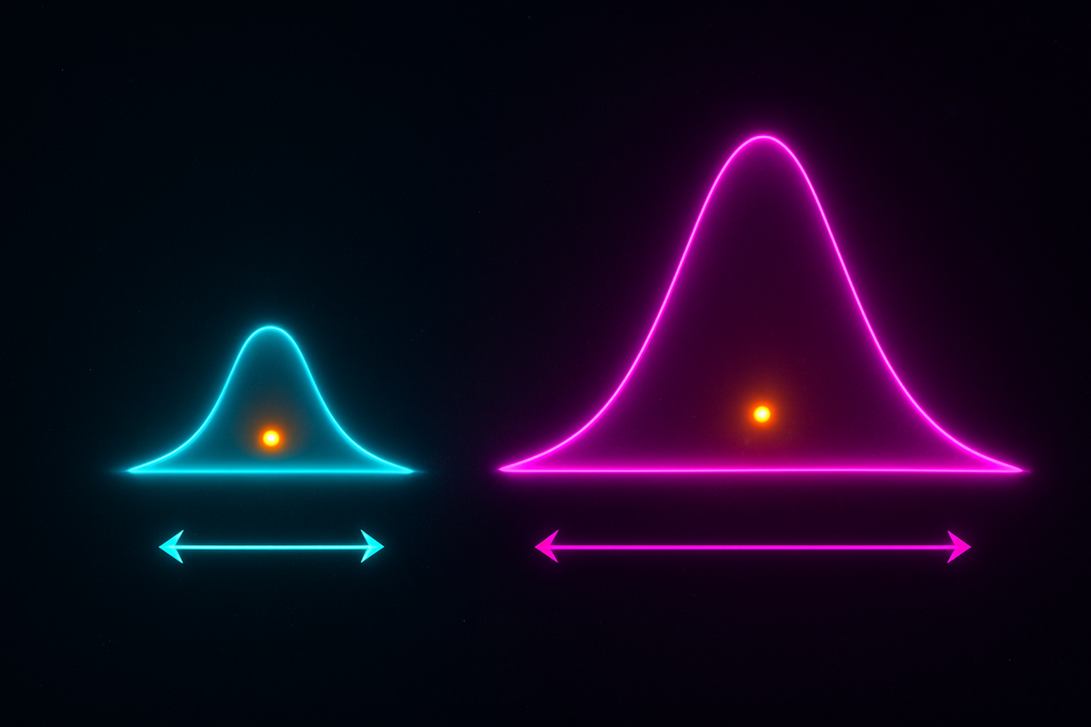
Variance captures this. It measures how spread out a distribution is—how much values deviate from the mean on average.

The Definition

Variance of a random variable X:

Var(X) = E[(X - μ)²]

where μ = E[X] is the mean.

In words: the expected squared deviation from the mean.

Expanded form:

Var(X) = E[X²] - (E[X])²

This is often easier to compute.

Standard deviation:

σ = √Var(X)

Standard deviation is in the same units as X. Variance is in squared units.

Computing Variance

Example: Fair die.

E[X] = 3.5 E[X²] = (1 + 4 + 9 + 16 + 25 + 36)/6 = 91/6 ≈ 15.17 Var(X) = 91/6 - (3.5)² = 91/6 - 12.25 = 91/6 - 73.5/6 = 17.5/6 ≈ 2.92 σ ≈ 1.71

Example: Bernoulli (coin flip, p = 0.5).

E[X] = 0.5 E[X²] = 0²(0.5) + 1²(0.5) = 0.5 Var(X) = 0.5 - 0.25 = 0.25 σ = 0.5

General Bernoulli:

Var(X) = p(1-p)

Maximum variance at p = 0.5.

Why Squared Deviations?

Why not just E[|X - μ|]—the mean absolute deviation?

Mathematical convenience. Squared deviations:

• Are differentiable everywhere
• Lead to elegant formulas
• Connect to the normal distribution
• Allow linear algebra (variance-covariance matrices)

Mean absolute deviation is sometimes used, but variance dominates for mathematical tractability.

Properties of Variance

Scaling:

Var(cX) = c² Var(X)

Double the random variable, quadruple the variance. This makes sense—deviations double, squared deviations quadruple.

Shifting:

Var(X + c) = Var(X)

Adding a constant doesn't change spread—just shifts the distribution.

Sum of Independent Variables:

If X and Y are independent:

Var(X + Y) = Var(X) + Var(Y)

Variances add for independent sums. This is crucial for the Central Limit Theorem.

Warning: For dependent variables, this fails. In general:

Var(X + Y) = Var(X) + Var(Y) + 2Cov(X, Y)

where Cov(X, Y) is the covariance.

Covariance and Correlation

Covariance:

Cov(X, Y) = E[(X - μₓ)(Y - μᵧ)] = E[XY] - E[X]E[Y]

Positive covariance: X and Y tend to be high or low together. Negative covariance: X high when Y low, and vice versa. Zero covariance: no linear relationship.

Correlation:

ρ(X, Y) = Cov(X, Y) / (σₓ σᵧ)

Correlation is covariance normalized to [-1, 1].

• ρ = 1: Perfect positive linear relationship
• ρ = -1: Perfect negative linear relationship
• ρ = 0: No linear relationship

Independence implies zero covariance, but not conversely. X and Y can have zero covariance while still being dependent.

Standard Deviation Intuition

Standard deviation is in the same units as the data.

A stock with σ = 15% has typical deviations of about 15% from expected return.

Chebyshev's Inequality:

For any distribution:

P(|X - μ| ≥ kσ) ≤ 1/k²

At least 75% of values are within 2 standard deviations. At least 89% are within 3 standard deviations.

For the normal distribution (more precise):

68% within 1σ 95% within 2σ 99.7% within 3σ

This is the famous "68-95-99.7 rule."

Common Variances

Bernoulli (p): Var = p(1-p)

Binomial (n, p): Var = np(1-p)

Poisson (λ): Var = λ (equals the mean!)

Uniform (a, b): Var = (b-a)²/12

Exponential (λ): Var = 1/λ²

Normal (μ, σ²): Var = σ² (by definition)

Variance of Sample Mean

If X₁, X₂, ..., Xₙ are independent with the same distribution (mean μ, variance σ²):

X̄ = (X₁ + X₂ + ... + Xₙ)/n

Then:

E[X̄] = μ Var(X̄) = σ²/n σ_X̄ = σ/√n

The variance of the sample mean decreases as sample size increases. This is why averaging works—it reduces variability.

This σ/√n is the standard error. It measures uncertainty in sample means.

Application: Risk

In finance, variance measures risk.

Modern Portfolio Theory:

Two assets with expected returns μ₁, μ₂ and variances σ₁², σ₂². A portfolio with weights w₁, w₂:

Expected return: w₁μ₁ + w₂μ₂ Variance: w₁²σ₁² + w₂²σ₂² + 2w₁w₂Cov(R₁, R₂)

If the assets are negatively correlated, portfolio variance can be less than either individual variance. This is diversification.

Sharpe Ratio:

(Return - Risk-free rate) / Standard deviation

Measures return per unit of risk. Higher is better.

Application: Measurement

In science, variance quantifies measurement uncertainty.

Error Propagation:

If Y = f(X) and X has small variance:

Var(Y) ≈ (f'(μₓ))² Var(X)

The variance of a function of a random variable depends on the derivative.

Weighted Averages:

If measurements have different uncertainties, weight by inverse variance. This minimizes total uncertainty.

Variance vs Entropy

Variance measures spread for real-valued variables.

Entropy measures spread for probability distributions more generally.

For the normal distribution, entropy depends on variance: H = ½ log(2πe σ²).

Higher variance → higher entropy → more uncertainty.

The Second Moment

Variance is E[X²] - (E[X])², related to the second moment E[X²].

Higher moments exist too:

• Third moment → skewness (asymmetry)
• Fourth moment → kurtosis (tail heaviness)

But variance is the most important. It appears in:

• The Central Limit Theorem
• Portfolio theory
• Error analysis
• Confidence intervals
• Regression

Understanding variance is essential to understanding uncertainty.

This is Part 7 of the Probability series. Next: "The Normal Distribution: Why the Bell Curve Is Everywhere."

Part 7 of the Probability series.

Previous: Expected Value: The Long-Run Average Next: The Normal Distribution: The Bell Curve and Why It Appears Everywhere