Synthesis: Vector Calculus as the Language of Physics
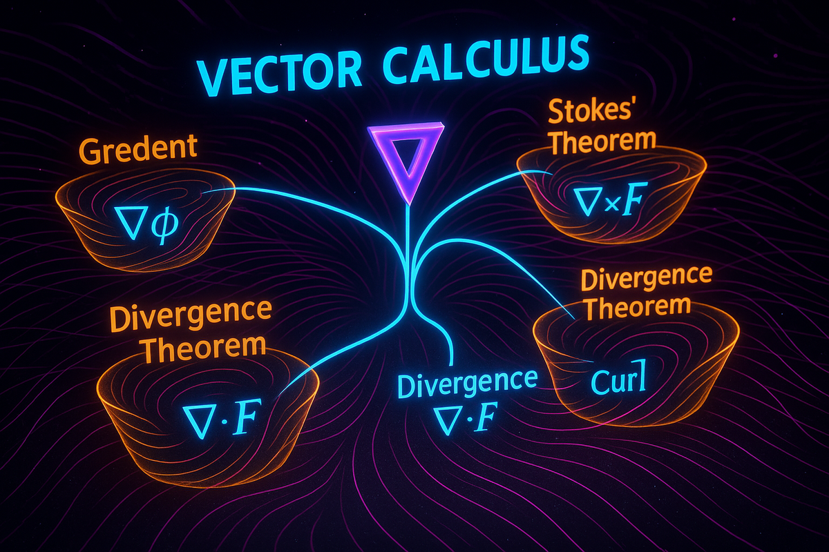
Gradient tells you which way a field climbs. Divergence tells you if it's spreading out or converging. Curl tells you if it's rotating. Together, these three operators let you write Maxwell's equations, Navier-Stokes, and almost every other law of classical physics.
Vector calculus is not a collection of techniques. It's a unified mathematical framework with three core components that interlock perfectly. Once you see how they connect, the whole structure crystallizes.
The components:
- Vector fields — functions that assign vectors to points in space
- Differential operators — gradient, divergence, curl, unified by del (∇)
- Fundamental theorems — Green's, Stokes', Divergence, connecting local and global
Each component depends on the others. Vector fields are the objects. Differential operators measure their local properties. Fundamental theorems relate those local properties to global integrals over boundaries.
Together, they form the mathematical language for describing any continuous phenomenon involving direction: flow, force, flux, propagation, diffusion. This is why vector calculus appears in every domain of physics and engineering.
The Objects: Vector Fields
Everything starts with vector fields. A vector field F assigns a vector to every point in space:
F(x, y, z) = (P(x, y, z), Q(x, y, z), R(x, y, z))
This is how you describe anything that has magnitude and direction at every location. Velocity fields in fluids. Force fields in mechanics. Electric and magnetic fields in electromagnetism. Heat flux in thermodynamics.
Scalar fields (temperature, pressure, potential) are related but different. They assign numbers to points, not vectors.
The key shift in moving from regular calculus to vector calculus is thinking in terms of fields: functions defined everywhere in space, not just along a curve or on a grid of points.
The Local Operators: Gradient, Divergence, Curl
Three differential operators extract local properties from fields:
Gradient (∇φ) takes a scalar field φ and produces a vector field pointing in the direction of steepest increase. It's the fundamental operator connecting scalar and vector fields.
Divergence (∇ · F) takes a vector field and produces a scalar field measuring spreading. Positive divergence means the field is radiating out (sources). Negative means converging (sinks). Zero means balanced flow.
Curl (∇ × F) takes a vector field and produces a vector field measuring rotation. The direction of curl is the axis of rotation. The magnitude is the strength.
All three are built from the del operator ∇ = (∂/∂x, ∂/∂y, ∂/∂z):
- Gradient: ∇ acting on a scalar
- Divergence: ∇ dotted with a vector
- Curl: ∇ crossed with a vector
This notation reveals the algebraic unity. You're not learning three separate operators—you're learning one operator (∇) that acts in three different ways.
The Connections Between Operators
The operators are related by fundamental identities:
∇ × (∇φ) = 0: Curl of a gradient is always zero. Gradients are curl-free (irrotational).
∇ · (∇ × F) = 0: Divergence of a curl is always zero. Curls are divergence-free (solenoidal).
∇ · (∇φ) = ∇²φ: Divergence of gradient is the Laplacian, measuring curvature.
These aren't arbitrary facts—they're consequences of treating ∇ as a vector and applying dot and cross product identities.
The identities have profound implications:
- Conservative fields (F = ∇φ) have zero curl. They're path-independent.
- Divergence-free fields (∇ · F = 0) can be written as curls. They're solenoidal.
- Any field can be decomposed into a gradient part and a curl part (Helmholtz decomposition).
The operators aren't independent. They form a coherent algebraic structure.
The Global Integrals: Line, Surface, Volume
To connect local differential properties to global behavior, you need integration:
Line integrals (∫_C F · dr) sum a vector field along a curve. They measure work, circulation, voltage—anything accumulated along a path.
Surface integrals (∫∫_S F · dS) sum a vector field over a surface. They measure flux—how much field crosses the surface.
Volume integrals (∫∫∫_V f dV) sum a scalar field over a volume. Standard multivariable calculus.
These extend the basic integral to structured domains: curves, surfaces, volumes embedded in 3D space.
The key conceptual shift: you're no longer integrating over intervals [a, b]. You're integrating over geometric objects—paths that wind through space, surfaces that bend, volumes with complex boundaries.
The Fundamental Theorems: Connecting Local and Global
The three fundamental theorems are the heart of vector calculus. They all have the same structure: a del operation integrated over a region equals a boundary integral.
Green's Theorem (2D): ∫_C F · dr = ∬_R (∇ × F) dA
Line integral around a closed curve = double integral of curl over the region inside.
Circulation around the boundary = total rotation inside.
Stokes' Theorem (3D): ∫_C F · dr = ∫∫_S (∇ × F) · dS
Line integral around a curve = surface integral of curl over any surface with that curve as boundary.
Circulation around the edge = total rotation through the surface.
Divergence Theorem (3D): ∫∫_S F · dS = ∫∫∫_V (∇ · F) dV
Surface integral over a closed surface = volume integral of divergence inside.
Flux through the boundary = total spreading inside.
These theorems generalize the fundamental theorem of calculus (∫ f' = f(b) - f(a)). Instead of relating derivatives to differences at endpoints, they relate del operations to boundary integrals.
They transform hard integrals into easier ones. They reveal conservation laws. They connect local properties (curl at a point, divergence at a point) to global behavior (circulation around a loop, flux through a surface).
The Unified Pattern
All three theorems follow the same template:
∫{boundary} (field) = ∫{interior} (del operation on field)
The boundary is one dimension lower than the interior:
- Green's: 1D boundary (curve), 2D interior (region)
- Stokes': 1D boundary (curve), 2D interior (surface)
- Divergence: 2D boundary (surface), 3D interior (volume)
The del operation depends on context:
- Green's and Stokes': curl (rotation sums to circulation)
- Divergence: divergence (spreading sums to flux)
This pattern extends infinitely. In differential geometry, there's a generalized Stokes' Theorem: ∫M dω = ∫{∂M} ω, where ω is a differential form and d is the exterior derivative. Green's, Stokes', and Divergence are all special cases.
The fundamental theorem of calculus is also a special case. The pattern is universal.
How Vector Fields Behave
Combining operators and theorems, you can classify vector fields:
Conservative fields (F = ∇φ):
- Curl is zero: ∇ × F = 0
- Line integrals are path-independent
- Circulation around closed loops is zero
- Examples: gravity, electrostatics
Solenoidal fields (∇ · F = 0):
- Can be written as curl: F = ∇ × A
- Flux through closed surfaces is zero
- Field lines form closed loops or extend to infinity
- Examples: magnetic field, incompressible fluid flow
General fields:
- Helmholtz decomposition: F = -∇φ + ∇ × A
- Sum of a conservative part and a solenoidal part
- Every field decomposes this way (uniquely, with boundary conditions)
This classification is fundamental. It reveals the structure of field theory.
Maxwell's Equations: The Synthesis
Maxwell's equations demonstrate the full power of vector calculus:
∇ · E = ρ/ε₀ ∇ · B = 0 ∇ × E = -∂B/∂t ∇ × B = μ₀J + μ₀ε₀∂E/∂t
Two divergence equations (sources). Two curl equations (dynamics and rotation).
The equations couple E and B through time derivatives. A changing B creates curling E (Faraday). A changing E creates curling B (Ampère-Maxwell). This feedback loop produces electromagnetic waves.
Every tool from vector calculus appears:
- Divergence measures charge density and the absence of magnetic monopoles
- Curl describes induction and current-driven magnetic fields
- Stokes' Theorem connects integral and differential forms of Faraday's and Ampère's laws
- Divergence Theorem connects integral and differential forms of Gauss's law
- Wave equation (∇²E = μ₀ε₀ ∂²E/∂t²) emerges from combining curl operations
Maxwell's equations are vector calculus distilled. Four lines that unify electricity, magnetism, and light.
Why the Framework is Coherent
Vector calculus isn't ad hoc. The pieces fit together for deep reasons:
Geometric origin: The operators measure geometric properties—steepness (gradient), spreading (divergence), rotation (curl). These are intrinsic properties of fields, not arbitrary definitions.
Algebraic structure: Del is a vector-like operator. Gradient, divergence, and curl emerge from applying vector operations (multiplication, dot product, cross product) to del. The identities follow from vector algebra.
Topological foundation: The fundamental theorems are about boundaries. A region's boundary is one dimension lower. The theorems connect integrals over regions to integrals over their boundaries. This is a topological fact, independent of coordinates.
Physical relevance: Nature seems to be described by fields and local differential equations. Conservation laws, wave equations, diffusion equations—all use divergence, curl, and Laplacian. The mathematics mirrors the physics.
This coherence is why vector calculus is teachable. It's not a bag of tricks. It's a unified system with clear structure.
The Learning Arc
Understanding vector calculus means climbing through levels:
Level 1: Computation You can calculate gradient, divergence, curl. You can set up and evaluate line integrals, surface integrals. You can apply the fundamental theorems to transform integrals.
This is mechanical. Necessary, but not sufficient.
Level 2: Geometric Intuition You understand what the operators measure. Gradient points uphill. Divergence detects sources. Curl detects rotation. Line integrals accumulate along paths. Surface integrals measure flux.
You can visualize fields and predict what operations will yield.
Level 3: Conceptual Unity You see how the pieces connect. Conservative fields are gradients. Solenoidal fields are curls. Fundamental theorems relate local to global. Maxwell's equations are four del operations.
You understand why the framework exists and how it encodes physical laws.
Level 4: Structural Insight You recognize vector calculus as a special case of differential geometry. You see connections to topology (homology, cohomology), gauge theory (connections, curvature), and functional analysis (Sobolev spaces, weak derivatives).
You understand the abstraction that unifies all the theorems.
Most people stop at Level 1 or 2. Getting to Level 3 is the goal of this series. Level 4 is graduate mathematics, but glimpsing it makes everything else make sense.
Why Vector Calculus Matters
Vector calculus is the language of continuous physics. Every classical field theory—electromagnetism, fluid dynamics, heat transfer, elasticity, general relativity—is formulated in vector calculus (or its generalization, tensor calculus).
Quantum mechanics uses operators on Hilbert spaces, but the Schrödinger equation involves the Laplacian. Quantum field theory quantizes classical fields—and those classical fields are described by vector calculus.
Engineering applications are ubiquitous. Antenna design, circuit theory, aerodynamics, heat exchangers, structural analysis—all require vector calculus.
Computational physics and engineering rely on discretizing vector calculus operators. Finite element methods, computational fluid dynamics, electromagnetic simulations—all based on approximating gradients, divergences, and curls on meshes.
If you work with anything that flows, propagates, diffuses, or exerts force, you need vector calculus.
The Beauty
There's an aesthetic dimension here. Maxwell's four equations unifying electromagnetism. The fundamental theorems connecting local and global. The del operator generating gradient, divergence, and curl through algebraic operations.
This isn't just useful. It's beautiful. The mathematics reflects deep structure in the physical world. The notation reveals unity that would be hidden in component form.
Gibbs and Heaviside, who developed modern vector notation, weren't just making calculations easier. They were making the structure visible. Before vector calculus, Maxwell's equations were 20 scalar equations. After, they're four vector equations. The compression reveals the pattern.
This is what good mathematical notation does. It doesn't just abbreviate—it clarifies. It makes the invisible visible.
The Next Steps
Vector calculus is a foundation, not an endpoint.
Tensor calculus generalizes vectors to tensors—objects with multiple indices that transform covariantly. General relativity requires tensor calculus to describe spacetime curvature. Continuum mechanics uses tensors for stress and strain.
Differential forms provide a coordinate-independent framework for integration and the fundamental theorems. They unify vector calculus with topology and reveal deeper structure. If you study differential geometry or mathematical physics, you'll encounter forms.
Geometric algebra (Clifford algebra) subsumes vector calculus into a more unified algebraic system. The dot and cross products are special cases of the geometric product. Some argue this should replace vector calculus in the curriculum.
Calculus of variations extends optimization to functionals—finding functions that minimize or maximize integrals. It connects to vector calculus through Euler-Lagrange equations and variational principles.
But for classical physics, engineering, and most applied mathematics, standard vector calculus is the tool. It's what working scientists use. It's what appears in textbooks. It's what you need to know.
The Payoff
After working through this series, you should be able to:
- Read Maxwell's equations and understand what each term means geometrically
- Recognize when a field is conservative or solenoidal
- Apply the fundamental theorems to transform integrals
- Understand why conservation laws have the form ∂ρ/∂t + ∇ · J = 0
- See the connection between differential and integral formulations of physical laws
- Visualize fields, sources, sinks, and vortices
- Appreciate why vector calculus is the natural language for field theory
This is mastery. Not just calculation, but understanding.
Vector calculus is one of those rare mathematical frameworks that's both theoretically elegant and practically indispensable. It unifies geometry, algebra, and analysis. It describes the physical world with remarkable precision. And it scales—from undergraduate physics to quantum field theory, the same operators and theorems reappear.
Learning it properly—understanding the geometric meaning, the algebraic structure, and the conceptual unity—is worth the effort. It changes how you see the world.
Fields aren't just functions. They're the texture of space. Gradient, divergence, and curl aren't just operators. They're the fundamental ways fields can behave. The theorems aren't just calculational tricks. They're statements about the relationship between local structure and global behavior.
This is the synthesis. Vector calculus is a coherent, beautiful, powerful framework for describing reality. Master it, and you've gained not just a tool, but a language—the language the universe seems to speak.
Part 12 of the Vector Calculus series.
Previous: Maxwell's Equations: Vector Calculus in Electromagnetism
Comments ()