What Is Multivariable Calculus? When Functions Have Multiple Inputs

The world doesn't happen in one dimension. Temperature across a room forms a field. Pressure in the atmosphere varies with altitude, latitude, and longitude. The trajectory of a thrown ball depends on initial velocity in three independent directions.

Single-variable calculus gave you the tools to analyze functions of one input: f(x). Multivariable calculus? That's where you graduate to functions of multiple inputs simultaneously: f(x, y) or f(x, y, z) or f(x₁, x₂, ..., xₙ).

This isn't just "calculus but with more variables." It's a conceptual leap into analyzing systems where change propagates through multiple dimensions at once, where geometry and algebra intertwine in ways that have no single-variable analogue.

The Core Shift: From Curves to Surfaces

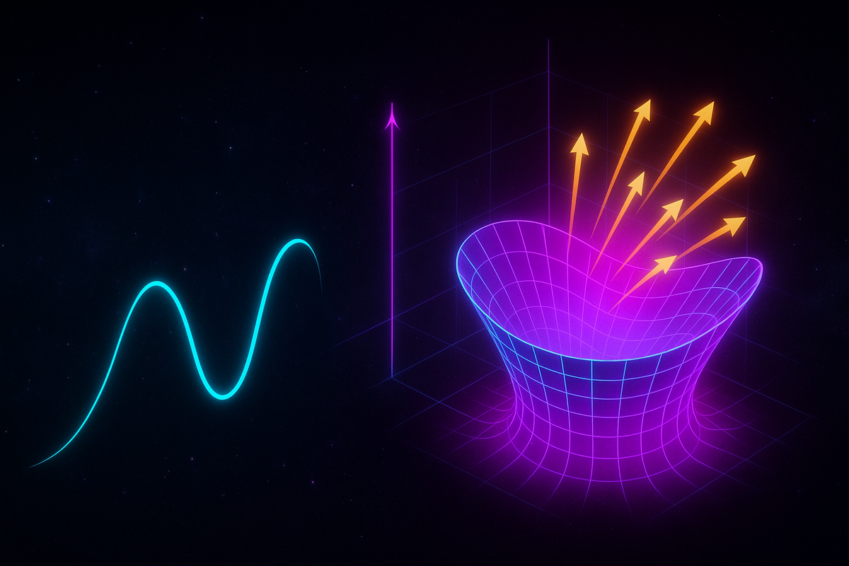
In single-variable calculus, you studied curves—graphs of y = f(x) living in two dimensions. The derivative df/dx told you the slope of that curve. The integral ∫f(x)dx gave you the area under it.

In multivariable calculus, even the simplest functions generate surfaces. Take z = f(x, y) = x² + y². That's not a curve—it's a paraboloid, a bowl-shaped surface extending in three dimensions. At every point on that surface, you can ask about slope, but now "slope" is direction-dependent. The surface rises steeply in one direction, gently in another.

This geometric richness is what makes multivariable calculus simultaneously harder and more interesting. You're not just doing algebra with more symbols—you're developing spatial intuition about how quantities vary across regions, how they flow through space, how they accumulate over volumes.

What Changes: Derivatives Become Directional

In single-variable calculus, there's only one way to take a derivative: df/dx measures how f changes as x increases. Done.

In multivariable calculus, you have choices:

Partial derivatives measure change in one direction while holding everything else constant. If f(x, y) represents temperature at position (x, y), then ∂f/∂x tells you how quickly temperature changes as you move east (increasing x) while staying at the same north-south position (constant y).

The gradient packages all partial derivatives into a vector that points in the direction of steepest ascent. It's not just a rate of change—it's a direction in space combined with a magnitude.

Directional derivatives measure the rate of change along any direction you specify. Want to know how temperature changes if you walk northeast at a 45-degree angle? The directional derivative tells you.

This proliferation of derivative concepts isn't complexity for its own sake. It reflects the geometric reality that surfaces have different slopes in different directions, and you need different tools to capture different aspects of that multidimensional variation.

What Changes: Integration Becomes Geometric

In single-variable calculus, ∫f(x)dx computes area under a curve—a region in 2D bounded by the curve and the x-axis.

In multivariable calculus, integration becomes inherently geometric:

Double integrals ∬f(x,y)dA compute volumes under surfaces—the space between a surface z = f(x, y) and the xy-plane. Or they compute total mass if f represents density. Or average temperature if f is a temperature field.

Triple integrals ∭f(x,y,z)dV accumulate quantities through three-dimensional regions. Mass of a solid with variable density. Total charge in an electromagnetic field. Heat energy in a volume of fluid.

The notation changes from dx to dA (for area elements) to dV (for volume elements) because you're integrating over regions of different dimensionality. The conceptual shift is from "area under a curve" to "accumulation over a region" to "total across a volume."

What Stays the Same: The Fundamental Questions

Despite the added dimensions, multivariable calculus asks the same core questions calculus always asks:

Differentiation: How does this quantity change? At what rate? In which direction?

Integration: How much is there in total? What's the aggregate effect across this region?

Optimization: Where are the maxima and minima? What configuration achieves the extreme value?

The techniques get more sophisticated—partial derivatives, gradient vectors, Lagrange multipliers—but the underlying intellectual move remains: analyze local behavior to understand global structure, break continuous variation into infinitesimal pieces you can sum back up.

The New Player: Vector Fields

Here's something genuinely new in multivariable calculus: vector fields. These are functions that assign a vector (not just a number) to every point in space.

Think of wind patterns: at every point in the atmosphere, there's a velocity vector indicating which direction the air is moving and how fast. That's a vector field.

Or electromagnetic fields: at every point in space, there's a vector indicating the direction and strength of the electric force. That's a vector field.

Vector fields introduce concepts with no single-variable analogue: divergence (how much the field is spreading out or converging), curl (how much the field is rotating), flux (how much of the field flows through a surface). These are the tools you need to describe fluid flow, electromagnetic phenomena, gravitational attraction—anything involving forces or flows in space.

Why Multiple Dimensions Aren't Just "More Work"

You might think multivariable calculus is just single-variable calculus done separately for each variable. It's not.

Coupling matters. In f(x, y) = x²y, the variables aren't independent—changing x affects how sensitive f is to changes in y. The mixed partial derivative ∂²f/∂x∂y captures this interaction.

Geometry constrains algebra. In single-variable calculus, all continuous functions look locally like straight lines (that's what "differentiable" means). In multivariable calculus, functions look locally like planes or curved surfaces, and the curvature in different directions can vary. Second derivatives form matrices, not numbers.

Topology emerges. In one dimension, you can only go left or right. In two or more dimensions, you can loop around obstacles, tie knots, encounter holes that aren't crossable. These topological features shape what calculus can and can't do—they're why certain theorems require closed curves or simply connected regions.

The extra dimensions create genuinely new mathematical structure, not just more of the same.

The Coordinate System Question

In single-variable calculus, you basically always use x as your variable. Done.

In multivariable calculus, choosing coordinates becomes a strategic decision. For a circle, Cartesian coordinates (x, y) force you to write x² + y² = r², which is algebraically messy. Polar coordinates (r, θ) let you write simply r = constant, which is geometrically natural.

Similarly:

• Cartesian (x, y, z) work for boxes and grids
• Cylindrical (r, θ, z) work for cylinders and tubes
• Spherical (ρ, θ, φ) work for spheres and radial symmetry

Changing coordinates isn't just relabeling—it's choosing the geometric framework that makes your problem tractable. The Jacobian determinant tells you how to convert integrals from one coordinate system to another, accounting for how volume elements get stretched or compressed.

This flexibility—analyzing the same function in different coordinate systems—is power you don't have in one dimension.

What Problems Multivariable Calculus Solves

Why learn this? Because the real world operates in multiple dimensions:

Physics: Electromagnetic fields, gravitational potentials, fluid dynamics, heat diffusion—all require multivariable calculus. Maxwell's equations are written in the language of vector calculus.

Engineering: Stress and strain in materials vary across three dimensions. Optimization of structures requires finding minima of functions with dozens or hundreds of variables.

Economics: Utility functions depend on multiple goods. Cobb-Douglas production functions relate output to labor and capital inputs. Optimization under budget constraints requires Lagrange multipliers.

Machine learning: Training a neural network means optimizing a loss function in a space with millions of dimensions. Gradient descent—literally following the gradient vector downhill—is how you find the minimum.

Computer graphics: Rendering realistic surfaces requires normal vectors, which are perpendicular to tangent planes, which are computed using partial derivatives. Ray tracing through 3D scenes uses parametric equations of lines in three-dimensional space.

You can't do modern science, engineering, economics, or data science without multivariable calculus. It's not optional background—it's the working language of quantitative analysis in higher dimensions.

The Learning Curve: What Makes It Hard

Multivariable calculus has a reputation for difficulty. Why?

Visualization is harder. In single-variable calculus, you can sketch y = f(x) easily. In multivariable calculus, even visualizing z = f(x, y) requires three-dimensional imagination. Functions of three or more variables can't be visualized at all—you need cross-sections, level sets, other proxy representations.

Notation proliferates. Partial derivatives ∂f/∂x, gradients ∇f, directional derivatives Dᵤf, Jacobian matrices, multiple integrals with varying differential notations (dA, dV, dS)—the symbolic landscape gets dense.

Theorems have more conditions. In single-variable calculus, a function is integrable if it's continuous (basically). In multivariable calculus, you need to specify the region's boundary, check whether it's closed or open, verify orientation for surface integrals—the geometric details matter.

But here's the thing: the difficulty comes from genuine richness. You're not just memorizing more formulas—you're developing geometric intuition about how functions behave in space, how changes propagate through systems, how integrals accumulate contributions over regions with complex shapes.

The Payoff: Thinking in Systems

The real value of multivariable calculus isn't computational—it's conceptual. It trains you to think about systems where multiple quantities vary simultaneously, where feedback loops create interdependencies, where optimization requires balancing competing constraints.

This is systems thinking mathematized. When you internalize the gradient as "direction of steepest ascent," you've developed an intuition that applies beyond mathematics: you can identify the direction of maximum improvement in any multi-parameter optimization problem.

When you understand how the Jacobian captures how small changes in inputs propagate to changes in outputs, you're equipped to analyze sensitivity in any coupled system—biological networks, economic models, engineering designs.

Multivariable calculus is training wheels for reasoning about complexity. The specific theorems matter less than the mental habits: decompose high-dimensional problems into manageable pieces, exploit symmetry to simplify coordinate systems, follow gradients to find extrema, integrate local information to recover global structure.

What's Next

This series will build multivariable calculus from the ground up:

• Partial derivatives for isolating change in one direction
• Gradients for finding steepest ascent
• Directional derivatives for change along arbitrary paths
• The multivariable chain rule for tracking dependencies
• Double and triple integrals for accumulation over regions and volumes
• Jacobians for changing coordinates
• Lagrange multipliers for constrained optimization

Each piece connects to the others, forming a coherent framework for analyzing functions of multiple variables.

By the end, you won't just know how to compute partial derivatives or set up double integrals. You'll have internalized a way of thinking about multidimensional systems—how to visualize them, how to differentiate them, how to integrate over them, how to optimize them.

That's the real prize: not facility with notation, but geometric intuition for how quantities vary across space, how changes propagate through dimensions, how the calculus of many variables reveals structure invisible in single-variable thinking.

Welcome to calculus as it actually operates in the world. Let's go.

Part 1 of the Multivariable Calculus series.

Previous: Multivariable Calculus Explained Next: Partial Derivatives: Rates of Change in One Direction