The Laplace Transform: Turning Calculus into Algebra
The Laplace transform is an escape hatch: transform a messy differential equation into algebra, solve it there, then transform back. It's one of the most elegant detours in all of applied mathematics.
The Laplace transform is sorcery. It converts differential equations into algebra.
Instead of solving dy/dt + 3y = e^(-2t) directly (calculus, integration, initial conditions), you transform it into sY(s) - y(0) + 3Y(s) = 1/(s+2) (algebra, solve for Y(s), transform back).
Differentiation becomes multiplication. Initial conditions plug in automatically. Solving becomes algebraic manipulation.
It's one of the most powerful techniques in differential equations, especially for engineering problems involving discontinuous forcing functions, impulses, and systems analysis.
What Is the Laplace Transform?
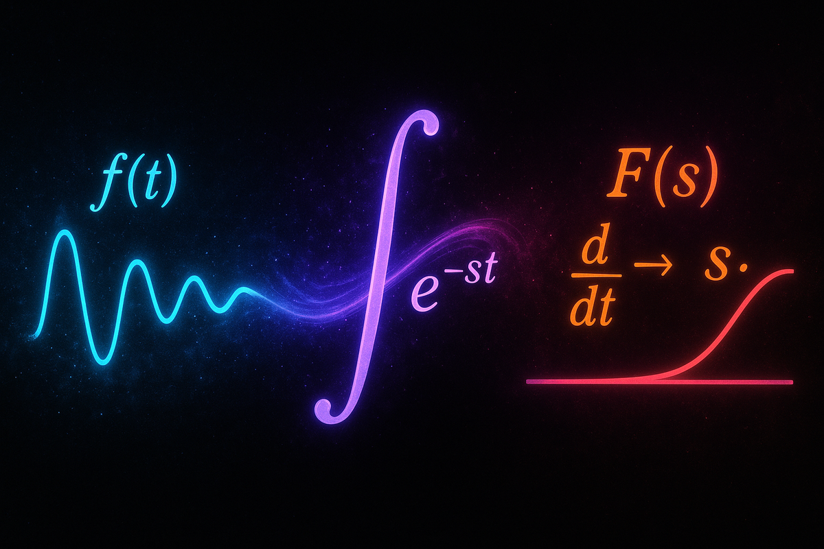
Given a function f(t) (defined for t ≥ 0), the Laplace transform is:
ℒ{f(t)} = F(s) = ∫₀^∞ e^(-st) f(t) dt
You integrate f(t) against the kernel e^(-st) from 0 to infinity. The result F(s) is a function of the complex variable s.
Key insight: The transform maps functions of time t to functions of frequency s. It's a change of domain—from time to frequency (or more precisely, complex frequency).
Why It Works
The magic: ℒ{df/dt} = sF(s) - f(0)
Differentiation in the time domain becomes multiplication by s in the frequency domain, minus the initial condition.
For second derivative:
ℒ{d²f/dt²} = s²F(s) - sf(0) - f'(0)
This converts differential equations into algebraic equations. Solve algebraically, then transform back.
Example: Basic Transform
Compute ℒ{e^(at)}.
F(s) = ∫₀^∞ e^(-st) e^(at) dt = ∫₀^∞ e^((a-s)t) dt
Evaluate (assuming s > a for convergence):
F(s) = [e^((a-s)t)/(a-s)]₀^∞ = 0 - 1/(a-s) = 1/(s-a)
So: ℒ{e^(at)} = 1/(s-a)
This is a fundamental transform pair.
Common Transform Pairs
| f(t) | F(s) = ℒ{f(t)} |
|---|---|
| 1 | 1/s |
| t | 1/s² |
| t^n | n!/s^(n+1) |
| e^(at) | 1/(s-a) |
| sin(ωt) | ω/(s²+ω²) |
| cos(ωt) | s/(s²+ω²) |
| e^(at)sin(ωt) | ω/((s-a)²+ω²) |
| e^(at)cos(ωt) | (s-a)/((s-a)²+ω²) |
These are the building blocks. Most problems reduce to combinations of these.
Transform of Derivatives
First derivative:
ℒ{f'(t)} = sF(s) - f(0)
Second derivative:
ℒ{f''(t)} = s²F(s) - sf(0) - f'(0)
nth derivative:
ℒ{f^(n)(t)} = s^n F(s) - s^(n-1)f(0) - s^(n-2)f'(0) - ... - f^(n-1)(0)
This is why Laplace transforms are powerful: derivatives become polynomial multiplication, and initial conditions appear explicitly.
Solving ODEs with Laplace Transform
Step 1: Take Laplace transform of both sides of the equation.
Step 2: Use linearity and transform of derivatives to convert to algebraic equation in F(s).
Step 3: Solve for F(s) algebraically.
Step 4: Use inverse Laplace transform (or table lookup) to find f(t).
Example: First-Order ODE
Solve: dy/dt + 3y = e^(-2t) with y(0) = 2
Step 1: Transform both sides.
ℒ{dy/dt} + 3ℒ{y} = ℒ{e^(-2t)}
sY(s) - y(0) + 3Y(s) = 1/(s+2)
Step 2: Substitute y(0) = 2.
sY(s) - 2 + 3Y(s) = 1/(s+2)
(s+3)Y(s) = 2 + 1/(s+2)
Step 3: Solve for Y(s).
Y(s) = 2/(s+3) + 1/((s+2)(s+3))
Partial fractions on second term:
1/((s+2)(s+3)) = A/(s+2) + B/(s+3)
1 = A(s+3) + B(s+2)
Set s = -2: 1 = A, so A = 1.
Set s = -3: 1 = -B, so B = -1.
Thus:
Y(s) = 2/(s+3) + 1/(s+2) - 1/(s+3) = 1/(s+3) + 1/(s+2)
Step 4: Inverse transform.
y(t) = ℒ⁻¹{1/(s+3)} + ℒ⁻¹{1/(s+2)} = e^(-3t) + e^(-2t)
Solution: y(t) = e^(-3t) + e^(-2t)
Check: Verify initial condition y(0) = 1 + 1 = 2. ✓
Differentiate: dy/dt = -3e^(-3t) - 2e^(-2t)
Substitute into ODE:
(-3e^(-3t) - 2e^(-2t)) + 3(e^(-3t) + e^(-2t)) = -3e^(-3t) - 2e^(-2t) + 3e^(-3t) + 3e^(-2t) = e^(-2t) ✓
Example: Second-Order ODE
Solve: y'' + 4y = 0 with y(0) = 1, y'(0) = 0
Step 1: Transform.
ℒ{y''} + 4ℒ{y} = 0
s²Y(s) - sy(0) - y'(0) + 4Y(s) = 0
Step 2: Substitute initial conditions.
s²Y(s) - s + 4Y(s) = 0
(s² + 4)Y(s) = s
Step 3: Solve for Y(s).
Y(s) = s/(s² + 4)
Step 4: Inverse transform (recognize as cosine).
y(t) = ℒ⁻¹{s/(s² + 4)} = cos(2t)
Solution: y(t) = cos(2t)
This is harmonic motion with ω = 2.
Linearity Property
The transform is linear:
ℒ{af(t) + bg(t)} = aℒ{f(t)} + bℒ{g(t)} = aF(s) + bG(s)
This means you can transform each term separately and combine.
Shifting Theorems
First shift (s-shift):
ℒ{e^(at)f(t)} = F(s-a)
Multiplying by exponential shifts the transform variable.
Example: ℒ{e^(3t)sin(2t)}
We know ℒ{sin(2t)} = 2/(s²+4).
Apply shift: ℒ{e^(3t)sin(2t)} = 2/((s-3)²+4)
Second shift (t-shift, Heaviside):
ℒ{f(t-a)u(t-a)} = e^(-as)F(s)
where u(t-a) is the Heaviside step function (0 for t < a, 1 for t ≥ a).
This handles delayed or shifted functions—critical for piecewise or impulse problems.
Heaviside Step Function
The unit step function:
u(t-a) = {0 if t < a; 1 if t ≥ a}
Transform: ℒ{u(t-a)} = e^(-as)/s
This models turning something on at time t = a.
Example: Switch turned on at t = 2, applying voltage V₀.
Voltage: V(t) = V₀ u(t-2)
Transform: ℒ{V(t)} = V₀ e^(-2s)/s
Dirac Delta Function
The impulse function δ(t-a) (infinite spike at t = a, zero elsewhere, unit area).
Transform: ℒ{δ(t-a)} = e^(-as)
This models instantaneous impulses—hammer blow, sudden force, electric pulse.
Example: Impulse at t = 0.
ℒ{δ(t)} = 1
An impulse at t = 0 transforms to a constant.
Convolution Theorem
For h(t) = (f * g)(t) = ∫₀^t f(τ)g(t-τ)dτ (convolution):
ℒ{f * g} = F(s)G(s)
Convolution in time domain ↔ multiplication in frequency domain.
This is critical for system analysis. If input is f(t), system response g(t), output is convolution f * g.
In Laplace domain: Output(s) = Input(s)·TransferFunction(s)
Transfer Functions
For a linear time-invariant system with input u(t) and output y(t):
Transfer Function = Y(s)/U(s)
This completely characterizes the system. Given any input, multiply by transfer function to get output.
Example: RC circuit.
Differential equation: dy/dt + (1/RC)y = (1/RC)u(t)
Transform (zero initial condition):
sY(s) + (1/RC)Y(s) = (1/RC)U(s)
Y(s)[s + 1/RC] = (1/RC)U(s)
Transfer function:
H(s) = Y(s)/U(s) = (1/RC)/(s + 1/RC) = 1/(RCs + 1)
This tells you: for any input U(s), the output is Y(s) = H(s)U(s).
Inverse Laplace Transform
Going from F(s) back to f(t) is the inverse Laplace transform:
f(t) = ℒ⁻¹{F(s)}
Techniques:
- Table lookup: Recognize F(s) as a standard form
- Partial fractions: Decompose rational functions
- Shifting theorems: Handle exponentials and delays
- Convolution: For products F(s)G(s)
Most practical problems reduce to partial fractions + table lookup.
Partial Fractions (Review)
For rational F(s) = P(s)/Q(s) (degree P < degree Q):
- Factor Q(s) into (s-a), (s-b), ..., (s²+bs+c), ...
- Decompose into sum of simple fractions
- Inverse transform each term using table
Example: F(s) = (3s+5)/((s+1)(s+2))
Partial fractions:
(3s+5)/((s+1)(s+2)) = A/(s+1) + B/(s+2)
3s+5 = A(s+2) + B(s+1)
Set s = -1: 2 = A, so A = 2.
Set s = -2: -1 = -B, so B = 1.
Thus:
F(s) = 2/(s+1) + 1/(s+2)
Inverse:
f(t) = 2e^(-t) + e^(-2t)
When Laplace Dominates
Laplace transforms shine for:
Piecewise functions: Heaviside steps and switches
Impulses: Delta functions (sudden forces, shocks)
Systems analysis: Transfer functions and frequency response
Engineering problems: Control systems, circuits, mechanical vibrations
For simple ODEs with continuous forcing, standard methods (integrating factor, characteristic equation) might be faster. But for complex forcing or systems, Laplace is king.
Limitations
Limitation 1: Only works for linear constant-coefficient ODEs. Nonlinear or variable-coefficient equations don't transform cleanly.
Limitation 2: Requires functions to grow slower than exponential (for convergence of transform integral). Most physical functions satisfy this.
Limitation 3: Inverse transform can require complex analysis (residue theorem) for non-standard forms.
Despite these, Laplace transforms are indispensable in engineering.
Comparison: Laplace vs Fourier
Fourier Transform: F(ω) = ∫_{-∞}^∞ f(t)e^(-iωt)dt
Real frequency ω, integrates over all time.
Laplace Transform: F(s) = ∫₀^∞ f(t)e^(-st)dt
Complex frequency s = σ + iω, integrates from 0 (causal systems).
Laplace generalizes Fourier. For s = iω (pure imaginary), Laplace reduces to Fourier (if function converges).
Fourier is for steady-state frequency analysis. Laplace handles transients and initial conditions.
Summary of Method
To solve ODE using Laplace:
- Take Laplace transform of equation (use derivative formula)
- Substitute initial conditions
- Solve algebraically for Y(s)
- Use partial fractions if needed
- Inverse transform using table or theorems
It converts calculus to algebra. The price: learning transform pairs and inverse techniques. The payoff: systematic method for complex forcing functions.
Next: Synthesis, where we tie everything together and see how differential equations model reality.
Part 11 of the Differential Equations series.
Previous: Systems of ODEs: When Multiple Quantities Change Together Next: Synthesis: Differential Equations as the Grammar of Physics
Comments ()