Ordinary vs Partial: ODEs and PDEs

The split between ordinary differential equations (ODEs) and partial differential equations (PDEs) isn't just mathematical bookkeeping. It's the difference between modeling change along one dimension versus modeling change across space and time simultaneously.

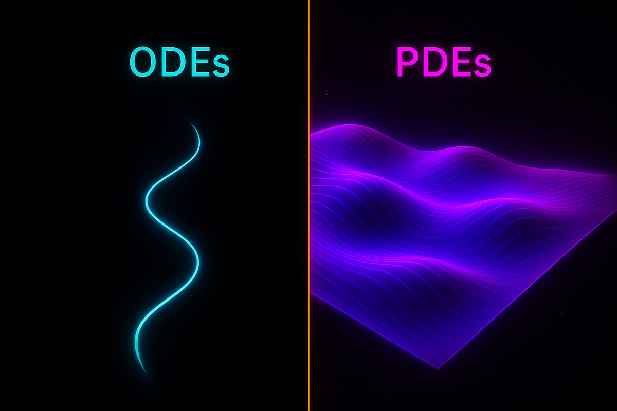
ODEs describe trajectories. PDEs describe fields.

That distinction unlocks entirely different classes of phenomena.

Ordinary Differential Equations (ODEs)

An ODE involves derivatives with respect to a single independent variable.

Example: dy/dx = y

Here y is a function of x alone. The derivative dy/dx tells you how y changes as x changes. One input variable, one output variable, one dimension of change.

Standard form: dy/dx = f(x, y)

The rate of change of y depends on x and possibly on y itself, but only on those. No other variables enter the picture.

Physical interpretation: ODEs model systems evolving along one dimension—usually time.

• Falling object: d²x/dt² = -g (position as a function of time)
• Radioactive decay: dN/dt = -λN (particle count as a function of time)
• Damped oscillator: m(d²x/dt²) + c(dx/dt) + kx = 0 (position as a function of time)

In each case, there's one independent variable (time) and the equation describes how the dependent variable evolves along that single dimension.

Partial Differential Equations (PDEs)

A PDE involves derivatives with respect to multiple independent variables.

Example: Heat equation ∂u/∂t = α(∂²u/∂x²)

Here u is temperature, which depends on both time t and position x. You have partial derivatives—rates of change with respect to one variable while holding others constant.

Standard form: Involves ∂u/∂t, ∂u/∂x, ∂²u/∂x², etc.

The notation ∂ (not d) signals partial differentiation: varying one variable while freezing others.

Physical interpretation: PDEs model fields evolving in space and time.

• Heat diffusion: temperature varying across space and evolving over time
• Wave propagation: displacement varying across space and oscillating over time
• Fluid flow: velocity field varying across three spatial dimensions and evolving over time

PDEs describe distributed systems where the state at each point depends on neighboring points.

The Key Difference

ODEs: Function of one variable. y(x) or y(t).

Solution is a curve—a one-dimensional trajectory.

PDEs: Function of multiple variables. u(x,t) or u(x,y,z,t).

Solution is a field—a function defined over space and time.

Think of it this way:

• ODE: "What's the trajectory of this particle?"
• PDE: "What's the pattern across this entire medium?"

Examples Compared

Exponential growth (ODE):

dP/dt = rP

Population P depends only on time. At each instant, the growth rate depends on current population. Solve to get P(t)—population as a function of time.

Diffusion (PDE):

∂u/∂t = α(∂²u/∂x²)

Concentration u depends on both position x and time t. At each point in space and each moment in time, the rate of change depends on the curvature of the concentration profile. Solve to get u(x,t)—concentration as a function of position and time.

The ODE gives you a timeline. The PDE gives you a spacetime field.

Why ODEs Are Easier

ODEs are hard. PDEs are harder.

Why? Because solutions to ODEs are curves in one dimension. Solutions to PDEs are surfaces (or hypersurfaces) in multiple dimensions.

An ODE typically reduces to integration—finding antiderivatives. Techniques exist: separation of variables, integrating factors, characteristic equations, series solutions.

A PDE requires satisfying conditions across entire spatial domains while evolving in time. Boundary conditions matter. Initial conditions matter. The geometry of the domain matters.

Many PDEs have no closed-form solutions. You need numerical methods (finite differences, finite elements, spectral methods) to approximate solutions on grids.

When to Use Each

Use ODEs when:

• System has one degree of freedom (one independent variable)
• Modeling point particles or lumped systems
• Time evolution without spatial variation
• Discrete components (like circuit elements or mechanical linkages)

Examples: Projectile motion, RC circuits, predator-prey dynamics, epidemiological SIR models, pendulum motion.

Use PDEs when:

• System has multiple degrees of freedom (multiple independent variables)
• Modeling continuous media or fields
• Spatial variation matters
• Distributed systems (like fluids, electromagnetic fields, vibrating membranes)

Examples: Heat conduction, wave propagation, fluid dynamics, electromagnetic fields, quantum mechanics.

Converting Between Them

Sometimes PDEs reduce to ODEs through symmetry or simplification.

Example: Heat equation in one dimension with no time dependence becomes an ODE.

Full PDE: ∂u/∂t = α(∂²u/∂x²)

Steady-state (∂u/∂t = 0): ∂²u/∂x² = 0

This is an ODE in x (even though we write ∂, it's only one variable). Solution: u = Ax + B, a straight line.

Example: Separation of variables converts PDEs into systems of ODEs.

Assume u(x,t) = X(x)T(t) (product of functions of single variables).

Substitute into heat equation:

X(T') = α(X'')T

Divide by XT:

T'/T = α(X''/X)

Left side depends only on t, right side only on x. Both must equal a constant. This gives two ODEs:

T' = -λαT X'' = -λX

Each is solvable by ODE techniques. Combine solutions to reconstruct u(x,t).

This is a standard PDE trick: decompose into ODEs, solve those, then recombine.

Dimensions of the Domain

ODEs operate in 1D domains (along time or a spatial coordinate).

PDEs operate in higher-dimensional domains:

• 1D space + time: Heat on a rod, waves on a string
• 2D space + time: Vibrating membrane, shallow water waves
• 3D space + time: Electromagnetic fields, fluid flow, diffusion in 3D

The dimension of the domain determines computational complexity. Solving a PDE in 3D requires discretizing three spatial dimensions—grids with millions or billions of points.

Classification of PDEs

Just as ODEs have order (first, second, etc.), PDEs have order and additional structure.

Order: Highest derivative appearing.

• First-order: ∂u/∂t + c(∂u/∂x) = 0 (transport equation)
• Second-order: ∂²u/∂t² = c²(∂²u/∂x²) (wave equation)

Type: Second-order linear PDEs split into three types based on characteristic behavior:

1. Elliptic: ∂²u/∂x² + ∂²u/∂y² = 0 (Laplace equation)
   • Describes equilibrium states
   • Boundary value problems
   • Example: electrostatic potential
2. Parabolic: ∂u/∂t = α(∂²u/∂x²) (heat equation)
   • Describes diffusion processes
   • Initial value problems
   • Example: heat spreading
3. Hyperbolic: ∂²u/∂t² = c²(∂²u/∂x²) (wave equation)
   • Describes wave propagation
   • Initial value problems
   • Example: vibrating string

This classification matters because each type requires different solution techniques and exhibits different physical behavior.

Linearity Still Matters

Like ODEs, PDEs split into linear and nonlinear.

Linear PDE: ∂u/∂t = α(∂²u/∂x²) (heat equation—linear in u and its derivatives)

Nonlinear PDE: ∂u/∂t + u(∂u/∂x) = 0 (Burgers equation—u multiplies its derivative)

Nonlinear PDEs are vastly harder. Many fundamental equations in physics are nonlinear:

• Navier-Stokes equations (fluid dynamics)
• Einstein field equations (general relativity)
• Nonlinear Schrödinger equation (quantum mechanics with interactions)

Some nonlinear PDEs exhibit chaos, shock formation, and other wild behavior that linear equations never show.

Boundary and Initial Conditions

ODEs need initial conditions: values of the function (and possibly derivatives) at a starting point.

PDEs need both:

Initial conditions: State of the system at t = 0 across all space. Example: initial temperature distribution u(x,0) = f(x).

Boundary conditions: Behavior at the edges of the spatial domain for all time. Example: temperature at the rod's ends u(0,t) = u(L,t) = 0.

Different boundary conditions give different solutions:

• Dirichlet: Specify the value on the boundary (e.g., u = 0)
• Neumann: Specify the derivative on the boundary (e.g., ∂u/∂x = 0, no flux)
• Mixed: Combination of both

Getting boundary conditions right is critical. Wrong boundaries = wrong physics.

Why PDEs Matter

Most real-world systems are spatially extended. Temperature isn't uniform—it varies from place to place. Sound doesn't exist at a point—it propagates through space. Electric fields don't sit still—they ripple and interact.

PDEs capture that spatial structure.

Without PDEs, you couldn't model:

• Weather systems (Navier-Stokes + thermodynamics)
• Electromagnetic radiation (Maxwell's equations)
• Quantum mechanics (Schrödinger equation)
• General relativity (Einstein field equations)
• Reaction-diffusion patterns (Turing patterns in biology)

Every field theory is a PDE. Every wave phenomenon is a PDE. Every diffusion process is a PDE.

The Toolkit Diverges

Because ODEs and PDEs are so different, solution methods diverge.

ODE techniques:

• Separation of variables (for special forms)
• Integrating factors
• Characteristic equations
• Laplace transforms
• Series solutions
• Numerical methods (Euler, Runge-Kutta)

PDE techniques:

• Separation of variables (to reduce to ODEs)
• Fourier series and transforms
• Green's functions
• Method of characteristics (for first-order)
• Finite difference methods
• Finite element methods
• Spectral methods

Some concepts carry over (linearity, superposition, characteristic equations), but the implementation differs radically.

What You Need to Know

For this series, we focus on ODEs. Why?

Because ODEs are foundational. You must master ODE techniques before tackling PDEs. The intuition you build solving ODEs—understanding order, linearity, initial conditions, solution families—transfers directly to PDEs.

PDEs are essentially infinite-dimensional ODEs. When you discretize a PDE numerically, you convert it into a (very large) system of ODEs.

So learning ODEs isn't a detour. It's the necessary foundation.

The Split

Here's the division:

ODE territory: Dynamical systems, mechanical systems, circuits, population models, chemical kinetics (well-mixed), control theory.

PDE territory: Heat flow, wave propagation, fluid dynamics, electromagnetism, quantum mechanics, general relativity.

Both matter. Both are hard. But ODEs come first.

Next: we dive into first-order ODEs, the simplest class of differential equations and the foundation for everything else.

Part 2 of the Differential Equations series.

Previous: What Is a Differential Equation? When Change Depends on the Current State Next: First-Order ODEs: The Simplest Differential Equations