Persistent Homology 101: Finding Features That Matter

Series: Topological Data Analysis in Neuroscience | Part: 2 of 9

You have a cloud of points. Maybe they're neurons firing at different rates. Maybe they're fMRI voxels correlated at different strengths. Maybe they're positions of particles in a simulation. Doesn't matter. You have points in high-dimensional space, and you need to understand what structure they contain.

This is where most methods give up. Traditional statistics can tell you about means, variances, correlations. Graph theory can tell you about connectivity patterns. But neither can tell you about the shape of your data—the holes, the voids, the cavities that exist not in any single point but in how the points relate to each other across scales.

Persistent homology can.

It's the mathematical microscope that reveals topological features hidden in data. And unlike most powerful mathematical tools, it's not actually that complicated once you strip away the jargon. You're about to understand the core technique that's revolutionizing neuroscience, materials science, genomics, and a dozen other fields.

Let's build it from the ground up.

The Problem: Noise vs. Signal at Different Scales

Imagine you're trying to understand the structure of a city by looking at the locations of all the buildings. From very far away—say, from a satellite—individual buildings blur together. You see only the overall footprint of the urban area. No detail, but also no noise. Just the big picture.

Now zoom in. Individual buildings become visible. Neighborhoods emerge. But so does noise—that empty lot between two blocks, that gap where a building is under construction, the park that breaks up the density. Are these features meaningful? Or are they accidents of measurement, artifacts of timing, noise that will disappear at a different scale?

Zoom in further still. Now you see individual rooms, individual walls. More structure appears. But also more noise. A missing window pane. A gap between bricks. Are these important? Do they tell you something about the structure of the city? Or are they just... cracks?

This is the fundamental problem TDA solves: distinguishing robust structural features from noise by tracking what persists across scales.

A crack in a wall appears at one zoom level and disappears at another—it's noise. A neighborhood void (a park, a lake, a plaza) appears when you zoom out a bit and remains visible across many scales—it's signal. The void defined by a city's highway loop persists across even more scales—it's definitely signal, a core organizing feature of the urban structure.

Persistent homology formalizes this intuition with mathematical precision. It builds geometric structures from your data at every possible scale simultaneously, then tracks which topological features appear at which scale and how long they last.

Features that persist are signal. Features that disappear quickly are noise.

Step 1: Building Simplicial Complexes

Start with your point cloud—let's say you've recorded from 100 neurons, and each neuron's firing rate at a particular moment gives you a point in 100-dimensional space. Over 10 seconds of recording, you have thousands of these points.

Now pick a radius—call it ε (epsilon). Draw a ball of radius ε around each point. Wherever two balls overlap, connect those points with an edge. Wherever three balls all mutually overlap, fill in a triangle. Where four balls overlap, fill in a tetrahedron. And so on, up to however many dimensions your data supports.

What you've built is called a Vietoris-Rips complex (or Rips complex for short). It's a geometric object assembled from your points according to a simple rule: connect things that are within ε of each other, and fill in all the higher-dimensional structures that result.

This geometric object has topology. It might have loops (1-dimensional holes). It might have voids (2-dimensional holes, like the surface of a sphere bounds empty 3D space). It might have higher-dimensional cavities that don't even have good visual intuition because they exist in four, five, ten dimensions.

But here's the key: the topology you get depends entirely on your choice of ε. Pick too small a radius, and nothing connects—you have isolated points, no structure. Pick too large, and everything connects—you have one giant blob, no interesting features. The meaningful structure exists somewhere in between.

So which ε do you choose?

Answer: all of them.

Step 2: The Filtration

Instead of picking one value of ε, you smoothly increase it from zero to infinity and watch what happens to your complex as it grows.

At ε = 0, you have just the points themselves. No edges, no triangles, nothing. Pure disconnection.

As ε increases slightly, edges start to form between nearby points. Clusters begin to emerge. Some points remain isolated longer—they're far from everything else.

ε increases more. The clusters merge. Triangles fill in. Loops might form—three or more points arranged in a circle with no point in the middle to fill the loop in.

ε continues growing. Those loops might fill in as more points get included. New loops might form. Voids might appear—regions enclosed by a shell of triangles with hollow space inside.

Eventually, ε gets large enough that everything connects into one giant high-dimensional blob. All structure is gone, swallowed by total connectivity.

This process—growing your complex continuously from empty to completely full—is called a filtration. You're filtering the data through increasingly coarse scales, watching structure appear and disappear.

Now comes the beautiful part: tracking which features appear when and how long they last.

Step 3: Birth, Death, and Persistence

Every topological feature—every connected component, every loop, every void, every higher-dimensional cavity—has a birth and a death.

A feature is born at the scale (the ε value) where it first appears in the filtration.

It dies at the scale where it gets filled in, merged, or otherwise destroyed.

The difference between death and birth is called the feature's persistence: how long it lasts across the range of scales.

Example 1: Connected components

At ε = 0, you have 100 separate points (assuming 100 neurons). That's 100 connected components. Each is born at ε = 0.

As ε increases, points start connecting. Two components merge into one. One of them (by convention, the younger one) dies at this ε value. The other survives, having absorbed its neighbor.

This continues—components merge, older ones absorb younger ones, the number of components decreases. Eventually, at some ε*, only one giant component remains. The last component to merge was the second-longest-lived component, dying when it merged into the oldest survivor.

The oldest component—the one that was born at ε = 0 and survived all the way to the end—has infinite persistence. It never dies (or you can say it dies when ε = ∞). This is meaningful: it represents the global connectivity of your dataset.

The second-oldest component has high but finite persistence. It represents a cluster that remained distinct for a long time before merging. This is signal—a real structural feature.

A component that's born at ε = 2.3 and dies at ε = 2.31 has tiny persistence. It's almost certainly noise—some random fluctuation in the spacing of your points.

Example 2: Loops (1-dimensional holes)

At small ε, no loops exist. As ε grows, suppose three points arranged in a triangle with empty space in the middle form a loop. This loop is born.

As ε continues to grow, maybe a fourth point inside the triangle gets included, filling in the loop. The loop dies.

The persistence of this loop is (death ε) - (birth ε). Long-lived loops are signal. Short-lived loops are noise.

Example 3: Voids (2-dimensional holes)

Maybe at some scale, your points form a shell—imagine a hollow sphere made of triangles. This creates a 2D void. It's born when the void first appears.

As ε grows, maybe the interior fills in with more points and triangles. The void dies.

Again: long persistence = signal, short persistence = noise.

This works in arbitrarily high dimensions. Your 100-neuron dataset can have 99-dimensional topological features. We can't visualize them, but the math doesn't care. Birth, death, and persistence work exactly the same way.

Step 4: Persistence Diagrams and Barcodes

How do you represent all this information? Two standard visualizations:

Persistence diagrams plot each feature as a point with (birth, death) coordinates. Features close to the diagonal (birth ≈ death) have low persistence—noise. Features far from the diagonal have high persistence—signal. The farther from the diagonal, the more important the feature.

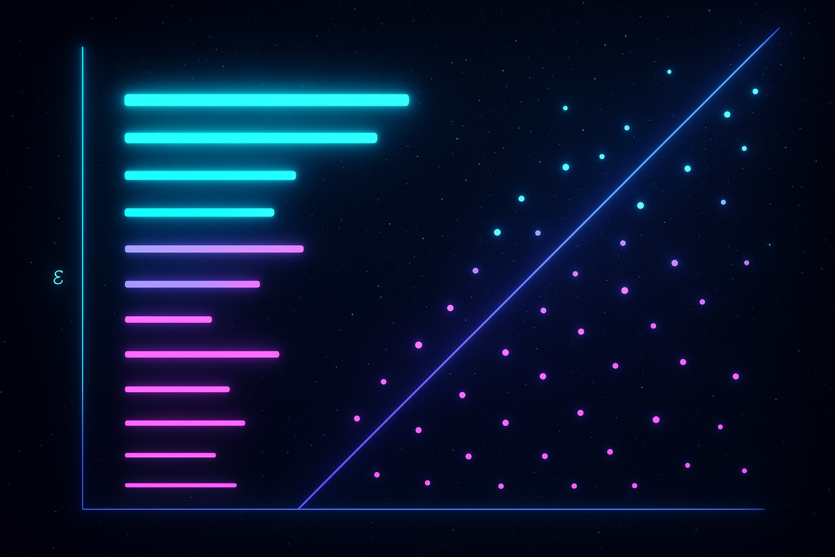
Barcodes show each feature as a horizontal line segment. The line starts at the birth scale and ends at the death scale. Long bars = persistent features = signal. Short bars = transient features = noise.

These visualizations make it immediately obvious which features matter. You can see at a glance the topological structure of your data across all scales simultaneously.

And here's what makes this powerful: you don't have to choose a scale. Traditional methods force you to pick a threshold—how similar do two things have to be before you call them "connected"? That choice determines everything you'll see. Pick wrong, and you miss the real structure or drown in noise.

Persistent homology sidesteps this entirely. It computes across all scales and tells you which features are robust across many scales. Those are the features that don't depend on arbitrary parameter choices. Those are the features that are actually there.

Why This Works for Brains

Neural data is disgustingly high-dimensional. Recording from 1,000 neurons gives you 1,000-dimensional state space. That's not a visualization problem—you can't visualize it, fine. That's a conceptual problem. What does it even mean to have structure in 1,000 dimensions?

Persistent homology gives you an answer: structure means topological features that persist across scales. And it doesn't matter how many dimensions you have. The math works in 3D, 300D, 3,000D exactly the same way.

When you apply this to neural activity, extraordinary patterns emerge:

Cognitive states have different topologies. Resting state, focused attention, memory recall—each creates different persistent features in the pattern of neural firing. You can literally see the difference in the barcode.

Learning reshapes topology. Before training, the neural activity has one topological structure. After training, it has another. The persistent features that characterize expertise are different from those characterizing novice performance. Mastery is visible in the geometry.

Disease disrupts topology. Alzheimer's progressively destroys persistent features. Depression flattens the topology. Schizophrenia creates incoherent features that don't integrate. You can measure the pathology geometrically.

Consciousness has a topological signature. The difference between conscious and unconscious states isn't just "more activity" or "different regions active." It's genuinely different topology—different persistent features, different Betti numbers (the counts of holes in each dimension), different geometric structure.

This is why TDA matters for neuroscience. Because the shape is the computation. And persistent homology is how you see the shape.

The Math You Can Skip (But Shouldn't Be Afraid Of)

For those curious about the formal machinery:

Homology is the algebraic tool that counts holes. In dimension 0, it counts connected components. In dimension 1, it counts loops. In dimension 2, it counts voids. In dimension k, it counts k-dimensional holes.

The k-th Betti number (denoted β_k) is the count of k-dimensional holes. β_0 = number of connected components, β_1 = number of loops, β_2 = number of voids, etc.

Persistence homology tracks how these Betti numbers change as you grow your complex through the filtration. Each feature contributes to β_k across the range of scales where it exists. The persistence diagram encodes this entire evolution compactly.

The beauty is that you can compute all this algorithmically. Software packages like GUDHI, Ripser, javaPlex, and Dionysus implement fast algorithms for extracting persistent homology from point cloud data. You feed in your points, you get back barcodes and persistence diagrams. The math stays hidden until you need it.

But even without the formalism, the intuition is simple: build geometry at every scale, track features that persist, distinguish signal from noise by how long features last.

That's it. That's persistent homology.

Practical Example: Visual Cortex Topology

Let's get concrete with real neuroscience. Researchers record from neurons in visual cortex while showing different images. Each image produces a pattern of neural activity—a point in the high-dimensional space of all possible firing patterns.

Show many images, get many points. Now apply persistent homology.

What do you find?

Different categories of images—faces, houses, objects, scenes—cluster in different regions of neural state space. But more than that: the topology of each cluster is different.

Faces might form a loop in state space—the neural representation of "faceness" has a 1-dimensional hole at its center. Maybe that hole corresponds to the "average face" that doesn't actually exist but that all actual faces orbit around.

Scenes might form higher-dimensional voids—the neural representation of spatial layouts has complex topological structure reflecting the geometric relationships between objects in the scene.

And here's the key: these topological features persist across different individual images within each category. They're robust. They don't depend on which specific face you show—the loop persists. They don't depend on threshold choices in your analysis—the features appear across many scales.

This is signal. This is how the brain organizes semantic categories geometrically. And you found it because you looked at topology instead of just activation levels.

Connection to Coherence Geometry

Everything we've described connects directly to AToM's framework:

Persistent features are coherent features. They maintain their identity across scales, across transformations, across perturbations. That's what coherence means—stable integration that resists dissolution.

Persistence is a measure of meaning. In M = C/T, persistence is the time component. Features that last across scales are features that carry information across transformations. They're the invariants that structure experience. They're where meaning lives.

Topological disruption is coherence collapse. When pathology destroys persistent features, it's destroying the geometric structure that enables integrated function. The manifold flattens. The holes disappear. Coherence fails. This isn't metaphor—it's measurable in the barcodes.

Recovery is topological repair. Therapy that rebuilds persistent features, medication that restores topology, practices that increase persistence—they're all working at the same level. They're restructuring the geometry of neural state space to recreate the features that enable function.

Persistent homology gives us mathematical tools to see what AToM claims exists: geometric structure that underlies coherent function. When that structure is robust across scales, the system works. When it fragments or flattens, pathology emerges.

The topology is the coherence. The persistence is the meaning.

This is Part 2 of the Topological Data Analysis in Neuroscience series, exploring how geometric methods reveal the hidden structure of mind.

Previous: The Shape of Thought: How Topologists Are Decoding the Brain
Next: The Blue Brain Project: Topology of Neural Circuits

Further Reading

• Edelsbrunner, H., & Harer, J. (2010). Computational Topology: An Introduction. American Mathematical Society.
• Ghrist, R. (2008). "Barcodes: The persistent topology of data." Bulletin of the American Mathematical Society, 45(1), 61-75.
• Carlsson, G. (2009). "Topology and data." Bulletin of the American Mathematical Society, 46(2), 255-308.
• Curto, C. (2017). "What can topology tell us about the neural code?" Bulletin of the American Mathematical Society, 54(1), 63-78.
• Sizemore, A. E., et al. (2019). "The importance of the whole: Topological data analysis for the network neuroscientist." Network Neuroscience, 3(3), 656-673.